How to Use VLOOKUP on Every Other Column in Google Sheets

Sometimes in Google Sheets, your data isn’t neatly arranged in adjacent columns. For example, sales figures, vendor quotes, or product categories may be spread across every other column. In such cases, a standard VLOOKUP cannot directly pull multiple non-adjacent values in one formula.

In this tutorial, you’ll learn how to:

Return values from every other column using VLOOKUP with an array of column indexes.
(Advanced) Search for a key across multiple non-adjacent columns when your data requires it.

By the end, you’ll have flexible formulas that handle both typical and complex scenarios, saving time and making your spreadsheets more dynamic.

Table of Contents

Return Values from Every Other Column Using VLOOKUP

Consider this list of items and their quoted prices from various vendors:

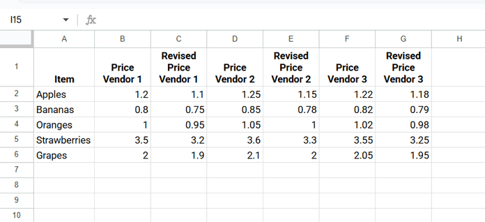
Sample Google Sheets data showing items and vendor prices, used to demonstrate VLOOKUP on every other column

Suppose you want to lookup an item, like “Oranges,” and return the revised prices from all vendors. The revised price columns are 3, 5, and 7.

=ARRAYFORMULA(IFERROR(VLOOKUP("Oranges", A2:G, {3, 5, 7}, FALSE)))

Result:

0.95   1.00   0.98

Making It Dynamic for Growing Columns

If you add more vendors in the future, you’d need to update {3,5,7}. Instead, you can make it dynamic using SEQUENCE:

=ARRAYFORMULA(IFERROR(VLOOKUP("Oranges", A2:G, SEQUENCE(1, COLUMNS(A2:G)/2, 3, 2), FALSE)))

SEQUENCE(1, COLUMNS(A2:G)/2, 3, 2) generates a sequence in 1 row, with as many columns as half of your range, starting from 3 and stepping by 2.
This ensures your formula automatically picks every other column, making it scalable for new vendors.

Advanced: Searching for a Key in Multiple Non-Adjacent Columns

Sometimes you need to search for a key in multiple non-adjacent columns and return a value from the column next to it. A standard VLOOKUP won’t work here.

Consider this dataset:

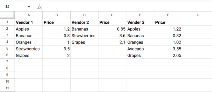
Google Sheets sample showing item prices from multiple vendors in non-adjacent columns

Suppose you want to find the prices of “Grapes” from all vendors.

⚠️ Tip: This data layout is not ideal. A better approach is to list each vendor below the previous one and use a separate column for vendor name, which allows FILTER to work cleanly.

Formula to Search Across Multiple Columns

=BYCOL(
    SEQUENCE(1, COLUMNS(A2:F)/2, 1, 2),
    LAMBDA(col, 
      VLOOKUP("Grapes", HSTACK(INDEX(A2:F, 0, col), INDEX(A2:F, 0, col+1)), 2, FALSE)
    )
)

Explanation:

SEQUENCE(1, COLUMNS(A2:F)/2, 1, 2) → selects every other column containing item names.
HSTACK(INDEX(...), INDEX(...)) → creates a temporary two-column array with the item and corresponding price.
VLOOKUP("Grapes", ..., 2, FALSE) → fetches the price for “Grapes” from that vendor column.
BYCOL(..., LAMBDA(...)) → repeats the search across all vendor columns.

This approach allows you to search for a key in non-adjacent columns and return values from the next column.

Sample Sheet

You can open this sample Google Sheet to test both scenarios:

Return values from every other column using VLOOKUP.
Search for a key across non-adjacent columns using BYCOL + HSTACK.

Tip: The sheet contains the sample datasets used in this tutorial so you can try the formulas directly and see the results in action.