In this tutorial, you’ll see how to use VLOOKUP in Google Sheets to find a value across multiple columns and return results from the associated row in a multi-column range. This reverse lookup technique lets you search for a value across columns (not just down a single column) and return a corresponding value from another column.

Let’s begin with a quick refresher on how VLOOKUP typically works, and then build up to the workaround needed for this more flexible use case.

Introduction to VLOOKUP in Google Sheets

As you may know, VLOOKUP has four parameters:

VLOOKUP(search_key, range, index, [is_sorted])

In the standard use case, the search_key must be in the first column of the range, and the formula looks down that column to return a value from another column in the same row.

Basic VLOOKUP Example in Google Sheets

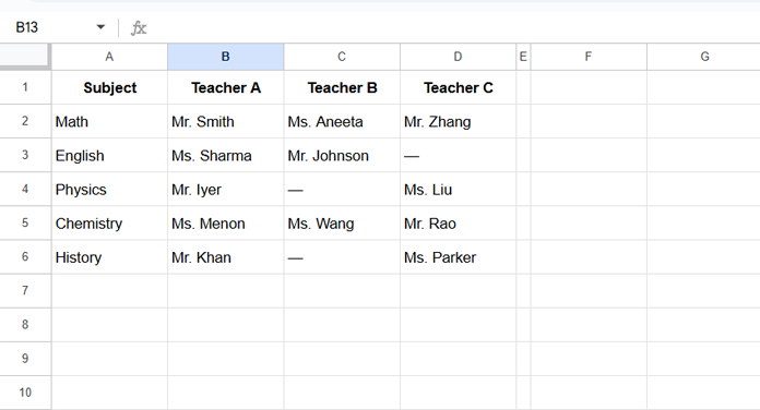
Suppose you have the following range A2:D, where:

• Column A contains subjects
• Columns B to D contain teacher assignments across different sections

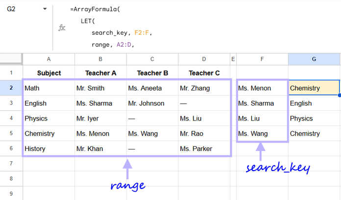
If cell F2 contains "Chemistry", this formula:

=ArrayFormula(VLOOKUP(F2, A2:D, {2, 3, 4}, FALSE))

…will return all three teachers assigned to Chemistry:

Ms. Menon, Ms. Wang, Mr. Rao

This is standard forward VLOOKUP behavior. But what if you want to do the reverse?

The Problem: Searching a Value Across Multiple Columns

What if you want to search for a teacher — for example, "Ms. Wang" — across columns B to D, and return the corresponding subject from column A?

That’s not something VLOOKUP supports directly, because it expects the search column to be first and doesn’t support searching across multiple columns. But we can solve it with a clever formula.

VLOOKUP Formula to Search Across Multiple Columns in Google Sheets

You can use the following array formula to search for a teacher’s name across multiple columns and return the associated subject.

=ArrayFormula(
   LET(
      search_key, F2:F, 
      range, A2:D,        
      blank, IFNA(WRAPCOLS(,ROWS(range))), 
      combine, TRANSPOSE(QUERY(TRANSPOSE(HSTACK(blank, CHOOSECOLS(range, 2, 3, 4), blank)),,9^9)), 
      vl, IF(search_key<>"", VLOOKUP("* "&search_key&" *", HSTACK(combine, CHOOSECOLS(range, 1)), 2, FALSE),), 
      vl
   )
)

This lets you search for a value across a matrix (columns B to D) and return the corresponding value from column A — even if you’re searching for multiple keys in F2:F.

How to Customize This Formula

Replace the ranges to suit your dataset:

• F2:F → your search key range
• A2:D → your full data range (including both search and result columns)
• CHOOSECOLS(range, 2, 3, 4) → the lookup columns (e.g., B, C, D)
• CHOOSECOLS(range, 1) → the result column (e.g., A)

Ready to test this formula with your own search keys?
Use the sample sheet as a starting point.

Formula Breakdown

Let’s break down how this works:

1. search_key

This refers to the values in F2:F — the teacher names you’re looking for.

We add spaces and wildcard asterisks like this:

"* " & search_key & " *"

This ensures partial matches work reliably, and avoids accidental substring matches (e.g., “Ms. Li” matching “Ms. Liu”).

2. combine – Flattening the Search Range

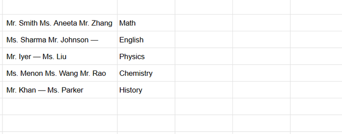
combine, TRANSPOSE(QUERY(TRANSPOSE(HSTACK(blank, CHOOSECOLS(range, 2, 3, 4), blank)),,9^9))

This transforms the selected columns (B to D) into a single column, where each row becomes a space-separated string like:

" Mr. Smith Ms. Aneeta Mr. Zhang "

This flattening technique — using TRANSPOSE + QUERY to combine multiple columns into a single-column array — is detailed in my tutorial: A Flexible Array Formula for Joining Columns in Google Sheets.

In this formula, we also add truly blank columns on both sides using
blank, IFNA(WRAPCOLS(, ROWS(range))). This ensures each row of combined values is padded with spaces, which helps avoid false partial matches when wildcard-searching with VLOOKUP.

3. Combining Lookup and Result Columns with HSTACK

HSTACK(combine, CHOOSECOLS(range, 1))

This combines the flattened lookup strings (teacher names) with the subject column, creating a two-column range suitable for VLOOKUP.

So we’re basically doing:

VLOOKUP(search_key, {flattened_teachers, subjects}, 2, FALSE)

4. Formula Output and Result Interpretation

If "Ms. Wang" is found in the flattened row " Ms. Menon Ms. Wang Mr. Rao ", VLOOKUP returns “Chemistry”, the subject in that row.

Features of This VLOOKUP Formula

• Works with multiple search keys (e.g., a list of teachers)
• Doesn’t use LAMBDA, so it’s more scalable for large datasets
• Searches across multiple columns, not just down a single one
• Can return 2D results if needed — just pass {2, 3} for multiple result columns

When to Use XLOOKUP Instead

If you want to do a similar lookup across columns but also:

• Search bottom to top
• Prefer a more readable structure

…then XLOOKUP may be a better fit. Here’s a detailed guide: How to Search Across Multiple Columns with XLOOKUP in Google Sheets

Related Resources

• Search Across Columns and Return the Header in Google Sheets
• Google Sheets: Find an Item’s Position Across Multiple Columns
• Retrieve Multiple Values Using VLOOKUP in Google Sheets