The purpose of using Named Ranges in Vlookup in Google Sheets is to make the formula looks cleaner. Other than this there are some hidden benefits that you will get when you use a combination of Vlookup and Named Ranges.
In this guide, you can learn all that benefits, I mean the benefits that came to my notice.
Vlookup is easy to learn if you understand the purpose of using it. I can easily connect Vlookup to outside of your Spreadsheet life.
For example, in Bus Terminals, Airports, Railway/Metro Stations you might have used your naked eye to find the information of a flight/train/bus arrival or departure time with the information that you have already in your hand.
Suppose you are in a metro rail station and you have the metro train number or name with you. You can probably use this information to find the train timing or route from the display panel at the metro station.
In Vlookup also we are doing the same. Here the display panel is the dataset, the information that you have is the search key.
You can name your dataset as for example “train_info”. It’s called Named Ranges. See how to use Named Ranges in Vlookup in Google Sheets.
I am going to include some additional tips on the use of Named Ranges in Vlookup like how a Named Ranges + Indirect + Vlookup combination works.
The Basic Use of Named Ranges in Vlookup in Google Sheets

Sample Data (Range A2: C5):
I have a price list of industrial items in the columns A, B, and C or you can say A2:C.
In that, column A contains the code of the items in Column B. You may already know why item codes are used.
It has several purposes like categorizing similar items and also it’s a part of warehouse tracking systems. Since it has nothing to do with our topic I am not going into that details.
The unit price of the items is in column C.
Search Key:
In cell E3 I have a search key that is the code of one item.
Expected Formula Output:
In cell F3 (please see the screenshot) I want to search this code (E3) in column A and if found return its unit price from column C.
I will show you how to use Vlookup to return the price without Named Ranges and also using Named Ranges.
Vlookup Without Named Ranges
Syntax:
VLOOKUP(search_key, range, index, [is_sorted])
Formula:
=vlookup(E3,A2:C5,3,0)
Generic Formula as an Explanation to the Vlookup Use:
vlookup(search key ["RBL1"] in cell E3,lookup range[A2:C5],column number that contains the price of item [3],exact match[0])
In this, you can replace the lookup range with Named Ranges. How?
Vlookup With Named Ranges
In the screenshot, you can see the Vlookup formula that uses the Named Ranges.
As you can see I have the price list of industrial items in the range A2: C5. It’s my lookup range in Vlookup. I am going to first name this range.
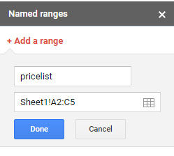
The name of my table is “pricelist” which covers the range A2: C5. How I have named this range for Vlookup? Here are the steps.
1. Select the data in the range A2: C5.
2. Click on the menu called “Data” and from the drop-down select “Named ranges…”
3. Type the name “pricelist” and click the button labeled as “Done”

Now let me show you how to use “pricelist” which is the newly created Named Ranges in Vlookup in Google Sheets.
Formula:
=vlookup(E3,pricelist,3,0)
This formula is the example to how to use Named Ranges in Vlookup in Google Sheets. In this, I have just replaced the lookup range A2: C5 with “pricelist”.
Find below two of the benefits of using Named Ranges in Google Sheets Vlookup and some advanced use of it.
The Main Benefits of Using Named Ranges in Google Doc Sheets
You can find below how using Named Ranges in Vlookup is beneficial in Google Sheets.
Use of Same Vlookup formula Across Sheet Tabs
For example;
My search key is in cell E3 in Sheet 5 and my source data containing the Named Range is in Sheet1.
Vlookup Formula with Named Ranges:
=vlookup(E3,pricelist,3,0)
Vlookup Formula without Named Ranges:
=vlookup(E3,Sheet1!A2:C5,3,0)
Now here is the main benefit of using Named Ranges in Vlookup in Google Sheets (first see the live screenshot at the bottom).
Switch Lookup Tables in Vlookup Using Drop-down Contains Named Ranges
In an earlier tutorial that related to Vlookup, I have shared how to switch the tables (range) in Vlookup using IF logical test – Examples to IF Vlookup Combination in Google Sheets.
Here is a more cool option. See how to use Named Ranges in Vlookup in Google Sheets to switch lookup tables.
Actually, this is a combination of Vlookup + Named Ranges + Indirect.
New to the Indirect function? Then follow this tutorial – Google Sheets Indirect Function Examples and Usage.
Let me take you to each step in detail. I have the following two tables. First, we must name it.

Named Ranges for Vlookup:
Name the range A3: B5 as “jennie” and D3: E5 as “allison”. I have already explained to you how to create Named Ranges for Vlookup above.
In concise, select each range and name from Data > Named ranges.
Drop-down Menu for Vlookup:
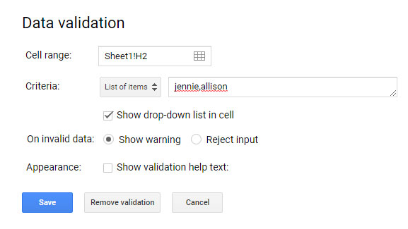
In cell H2, create a drop-down menu that contains the above two Named Ranges. Just follow the below instructions to create a drop-down for Vlookup in Google Sheets. We are using Data Validation feature here.
Go to the menu Data > Data Validation. There apply the below validation settings.

Now you have a drop-down menu in cell H2 which contains the already created table names as Named Ranges.
You are going to learn a different way of using Named Ranges in Vlookup in Google Sheets.
Search Key:
In Cell G2 enter the search key “Sedan”. Actually what we are going to do with this search key and drop-down is as follows.
I am going to apply one Vlookup formula in the cell I2. The formula will use the search key in G2 and Named Ranges in H2 to return the total sales quantity of the vehicle type “Sedan” either from the range B3: B5 or H3: H5.
The cell H2 drop-down actually contains two named ranges. But it’s a text string right now. With the help of the Indirect function, you can use cell H2 as Named Ranges.
So that, based on your selection of named ranges in the drop-down the lookup table in the Vlookup will get changed.
Vlookup + Named Range Drop-down + Indirect Combo:
The formula in cell I2:
=vlookup(G2,indirect(H2),2,0)
See this in action.

Does this formula support multiple search keys?
Yes! If you want to look up the total sales of Sedan and SUV, type Sedan in G2 and SUV in G3. Change the formula as below.
=ArrayFormula(vlookup(G2:G3,indirect(H2),2,0))
That’s all about the use of Named Ranges in Vlookup in Google Sheets. Enjoy!
Additional Resources:


