


You can create named ranges in Google Sheets to make your formulas cleaner and easier to read and understand. Named ranges are simply labels that you give to a cell or cell range.
You can use these labels in advanced formulas that involve Google Sheets functions like SUMIF, QUERY, VLOOKUP, and XLOOKUP.
For example, you could create a named range labeled gasoline_consumption for the table that contains your fleet’s gasoline consumption. You could then use the CHOOSECOLS function to select specific columns from this data for the XLOOKUP function.
I will show you an example of this at the end of this post.
Named Ranges in Google Sheets and Advantages of Using It
Ever wonder about seeing an unfamiliar function in a formula in Google Sheets?
It might be a formula that contains a named range, not a function.
Please check the table below, where you can see that cell range D4:D9 contain sales values.

How do you usually total them?
It might be as follows:
=SUM(D4:D9)But to make your formula cleaner and more user-friendly, you can first name the range D4:D9 as SalesValue and use it in your formula as follows:
=SUM(SalesValue)Another advantage of this is that you don’t need to remember the range D4:D9. Instead, you can memorize SalesValue and use it anywhere in the sheet (even in a different tab in that sheet).
How to Create a Named Range in Google Sheets
There are two ways to create a named range in Google Sheets. One is using the menu command, and another is using a shortcut method.
You may be unfamiliar with the latter method as it is relatively new.
Let’s see how to apply a name to the cell range D4:D9 using both methods.
Method 1: Using Menu Command
Here are the steps on how to create a named range in Google Sheets. It is the first step in making cleaner formulas.
- Select the cell range (
D4:D9, as per our example) that you want to name. - Go to the Data menu and click on Named ranges.
- In the Named Ranges sidebar panel, type a name for the range in the Name field. The field may already contain a suggested name
NamedRange1. You can overwrite it toSalesValue. - Click on the Done button.

Hereafter, in formulas in the same sheet (workbook), you can use the named range SalesValue instead of the range D4:D9.
Here are two examples:
=MAX(SalesValue)The above formula will return the maximum value in the named range SalesValue, which is the range D4:D9.
={SalesValue}The above formula will populate the data in the named range SalesValue, which is the range D4:D9, without processing it.
Method 2: Using Shortcut Keys
Here is the quickest way to create a named range in Google Sheets:
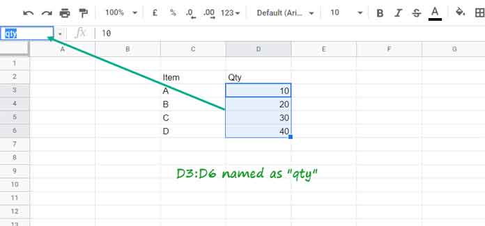
- Select the cell range (for example,
D3:D6). - Press the keyboard shortcut Ctrl + J on PC and ⌘ + J on Mac.
- Type the required name in the Name box.
Note: You can also directly click within the Name box and type the required name there.
Valid Names
Sometimes you may encounter the error message “The range name specified isn’t valid” when creating a named range in Google Sheets. Here are the possible reasons:
A valid named range must:
- Be 1 to 250 characters long.
- Only contain letters, numbers, and underscores (
_). - Not start with a number or the words (Boolean values) TRUE or FALSE.
- Not be a cell reference in A1 or R1C1 notation.
- Not contain spaces or punctuation.
How to Create a Named Range to a Table and Lookup It (Google Sheets)
Recall the gasoline consumption example that I mentioned at the beginning.
The gasoline consumption data is in the range A1:C100 and the field labels are Date, Vehicle Number, and Quantity in Gallon in cells A1, B1, and C1, respectively.
In short, the table is in the range A1:C100. Let’s create a named range pointing to this whole table and use it in XLOOKUP.
Name the range A1:C100 using one of the methods above. I prefer the name gasoline_consumption for this table.
The following formula will look up the vehicle number TEMP-DX-100 in the second column of the named range and return the matching value from the third column of it.
=XLOOKUP(
     "TEMP-DX-100",
     CHOOSECOLS(gasoline_consumption,2),
     CHOOSECOLS(gasoline_consumption,3)
)
Points to be Noted
When you insert a row or rows within the named range area, they will automatically be added to the range.
As per the above example, if you insert a row after row 10, the range reference would change from A1:C100 to A1:C101.
If you insert a row before the first row or after the last row of a named range in Google Sheets, it will not be included automatically.
Inserting a row above row 1 will move the named range from A1:C100 to A2:C101. You must edit the named ranges to include such additional rows.
The above points are also applicable to columns.
That means the named range is not fully dynamic. But there are workarounds to this problem.
- Auto-Expand Named Ranges in Google Sheets to Accommodate New Rows.
- Dynamic H&V Named Range in Google Sheets.
Use named ranges in Google Sheets to make your formulas look cleaner.