You can use named ranges in the ‘data’ argument of the QUERY function in Google Sheets. But what about replacing column identifiers like A, B, and so on?

To replace column identifiers with named ranges in the SELECT, WHERE, GROUP BY, ORDER BY, PIVOT, ORDER BY, LIMIT, OFFSET, LABEL and FORMAT clauses, you need to follow a workaround. This is useful because you can assign a name to a column (for example, “age”) and use that instead of a column ID.

Let me guide you through some examples of using named ranges in the QUERY data and the QUERY string.

Example of Using Named Ranges in QUERY Data

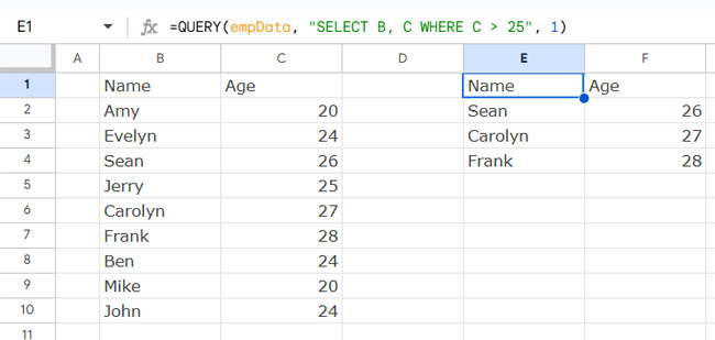
Assume you have sample data in B1:C10, where the first column contains names and the second column contains ages. Let’s assign the range B1:C10 the name empData.

You can assign names in two ways. The easiest method is as follows:

1. Select B1:C10.
2. Click the Name Box located at the top-left corner of the sheet, just above the grid and to the left of the formula bar.
3. Type empData.

Now, you can use this named range as the data in the QUERY formula:

=QUERY(empData, "SELECT B, C WHERE C > 25", 1)

This formula will return all the employees whose age is greater than 25.

How to Use Named Ranges in the QUERY String

Next, let’s assign the name empName to B1:B10 and age to C1:C10 using named ranges. You can select these ranges individually and type the respective names in the Name Box as shown earlier.

However, the QUERY function does not recognize named ranges in the query string to represent columns, as it requires column identifiers such as A, B, C, or Col1, Col2, Col3.

Assume you want to use the named range empName in the SELECT clause of the QUERY function. For the regular formula, you would write:

=QUERY(empData, "SELECT B", 1)

You might attempt the following formula:

=QUERY(empData, "SELECT empName", 1)

This won’t work because QUERY requires column identifiers, not named ranges. Instead of directly specifying the named range empName, you should use this syntax:

"&CHAR(64 + COLUMN(named_range))&"

Replace the placeholder text named_range with the name you want to use—in this case, empName.

=QUERY(empData, "SELECT "&CHAR(64 + COLUMN(empName))&"", 1)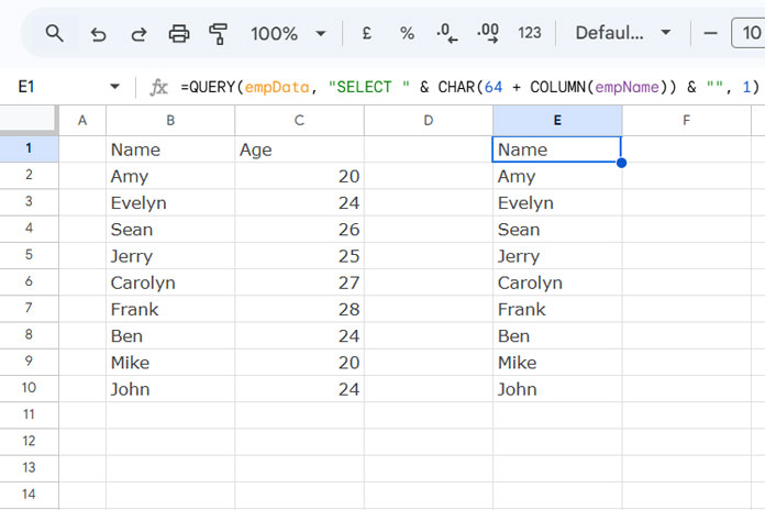

Now, let’s say you want to rewrite this formula:

=QUERY(empData, "SELECT B WHERE C > 25", 1)

Here, we are using both the SELECT and WHERE clauses.

You want to replace the column IDs B and C with the named ranges empName and age. You can replace B with "&CHAR(64 + COLUMN(empName))&" and C with "&CHAR(64 + COLUMN(age))&".

So, the final formula becomes:

=QUERY(empData, "SELECT "&CHAR(64 + COLUMN(empName))&" WHERE "&CHAR(64 + COLUMN(age))&" > 25", 1)

While the formula might seem complex, it’s easy to adapt once you understand the logic behind it.

How Does This Work?

Great question! Here’s the breakdown:

• The COLUMN function returns the column number of the named range. It’s not relative to the data but refers to the actual column number in the sheet.
• By adding 64 to the column number, we get the character code of the corresponding column.
• The CHAR function then converts that character code into the actual column ID, such as A, B, or C.

That’s the logic behind using named ranges in the QUERY function’s query string.

Resources

• Reference a Column by Field Label in Google Sheets QUERY
• Dynamic Column ID in QUERY with IMPORTRANGE Using Named Ranges
• Structured Table References in Formulas in Google Sheets