In this tutorial, we will discuss three scenarios where you may need to increment column references (identifiers) in QUERY formulas in Google Sheets:
- When you copy a QUERY formula to the right or left.
- When you delete any column within the data range.
- When you insert new columns.
By column reference, we mean the column identifiers in the query clauses. For example:
select A
select Col1
where B
where Col2
The column identifiers in Google Sheets QUERY may not move when you copy and paste a QUERY formula. This is because they are text strings, not cell references like A1, B1, etc. However, you can increment the columns in QUERY with a simple workaround.
You can make a column identifier relative in the Google Sheets QUERY function. This means that the column identifier will adjust when you copy the formula right or left, or when you delete or insert new columns in the data range.
Identifiers (IDs) in the QUERY function
We use column identifiers (IDs) to refer to columns within the QUERY function. The syntax of the QUERY function is as follows:
QUERY(data, query, [headers])Where:
datais the range of cells to be queried. Thedataargument in the QUERY function can be:- A physical range of cells (e.g., A1:Z1000)
- A named range (e.g., sales_data)
- An expression (e.g., {A1:Z1000} or IMPORTRANGE(spreadsheet_url, range_string))
queryis a string that specifies the query to be performed.headers(optional) is a range of cells that contains the header labels for the columns in the output of the QUERY function.
If you want to auto-increment columns when copying a QUERY formula or inserting or deleting one or more columns in the QUERY function data, you must first know how to specify columns correctly in the QUERY function.
Specifying IDs in the QUERY Function
There are two ways to specify columns in the QUERY function, depending on whether your data is a physical range, a named range, or an expression:
Physical range or named range: You can specify a column by its heading which is the heading that identifies a column of a sheet. They are labeled A, B, C, …, Z, and so on. For example, the following formula will select column C from the data in A1:D:
=QUERY($A$1:$D,"select C")Expression: You can specify a column by its number. The format is Col (It’s case-sensitive) followed by the column number. This is necessary because expressions do not have column headings. For example, the following formula will select column 5 from the data imported from another spreadsheet:
=Query({importrange("URL","Sheet1!A1:G")},"select Col5",1)You can make a physical range or named range into an expression by wrapping it in curly braces. This can be useful for auto-incrementing column references in QUERY. For example, the following formulas will select column 3.
=QUERY({$A$1:$D},"select Col3")  // physical range to expression
=QUERY({sales_data},"select Col3")  // named range to an expression
Note: Google Sheets started supporting column number identifiers with physical ranges. But we will stick with the curly braces approach because we are unsure whether there will be a rollback.
Incrementing Column References in QUERY SELECT Clause in Google Sheets
We will use an expression instead of a physical range or named range to auto-increment column references in QUERY.
To auto-increment a column reference in QUERY in Google Sheets, you can depend on the following syntax:
=QUERY({data},"select Col"&COLUMN(reference_cell))Where:
datais the range of cells to be queried.reference_cellis the first cell of the column that you want to increment or auto-adjust.
For example, the following formula will select the first column from the data range A1:D:
=QUERY({$A$1:$D}, "select Col"&COLUMN(A1))Please use absolute references in the data. Instead of A1:D you must use $A$1:$D.
Let’s see the explanation and the effect of this formula when we copy it to the right or left, delete a column from the data, or add a column to the data.
1. How to Auto-Increment Column References in QUERY When Copying to the Right
We have already seen the formula for auto-incrementing column references in the QUERY SELECT clause. Let me elaborate on it.
I have the following formula in cell F1:
=QUERY({$A$1:$D},"select Col"&COLUMN(A1))When I copy this QUERY formula to the right, it populates the second column, which means it increments the column references by one.

How does this formula increment the column in QUERY?
It’s a simple fix. Instead of the number 1 in Col1, I have used the COLUMN function.
The COLUMN(A1) function in the QUERY returns the number 1. I have concatenated the text select Col with it. So it becomes select Col1.
This makes the column reference flexible in QUERY. When you drag the formula to the right, the COLUMN(A1) function turns to COLUMN(B1), which obviously would return the number 2.
This helps us to increment the column in QUERY. If you copy the formula left, the column reference would of course decrease.
Now let us take a look at what happens to the above formula when we add or remove columns in the source data.
2. How to Move a Column Reference Automatically in QUERY When Deleting a Column
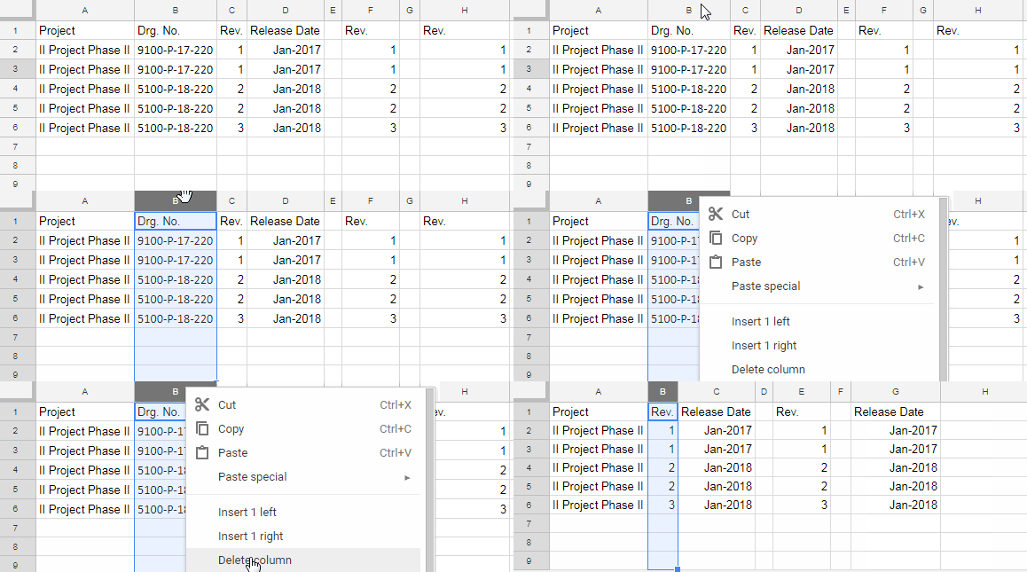
In the GIF below, you can see the following two QUERY formulas in action:
The formula in F1 that moves the column reference when column position changes:
=QUERY({$A$1:$D},"select Col"&COLUMN(C1))The conventional QUERY formula in H1 that stays constant:
=QUERY({$A$1:$D},"select Col3")
When I delete column B, the F1 formula retains the column values. The formula automatically adjusts to this change because the COLUMN(C1) function returns the column number of cell C1, which changes to B1 after column B is deleted. This ensures that the formula always retains the column values, regardless of whether columns are added or removed.
However, the conventional QUERY in cell H1 fails to retain the column values because the column identifier is constant in it. This means that the formula will always select the third column, even if columns are added or removed.
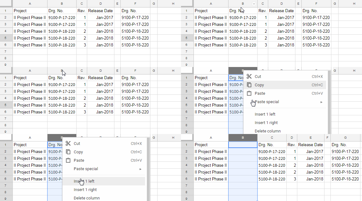
3. How to Auto Adjust a Column Reference in QUERY When Inserting a New Column
The data we are testing is in the range A1:D. Here is my dynamic formula that adjusts column identifiers automatically:
=QUERY({$A$1:$D},"select Col"&COLUMN(B1))This formula is currently in cell F1, which will populate the column B values. If I insert a new column between columns A and B, the formula will automatically increment the column in QUERY.
The position of the data in the second column moves to the third. Accordingly, the change is reflected in our formula. COLUMN(B1) becomes COLUMN(C1).

Incrementing Column References in QUERY WHERE and Other Clauses
Let’s code another QUERY formula that involves the SELECT and WHERE clauses. This will give you a general idea of how to increment column references in all the clauses in QUERY.
You May Like: What is the Correct Clause Order in Google Sheets Query?
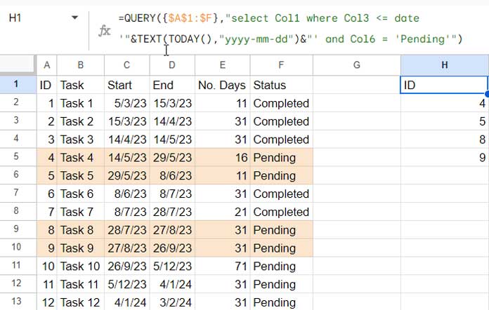
We have the following data in A1:F:

The following formula in cell H1 returns task IDs if the task start dates in column C are less than today’s date and the status is “Pending”.
=QUERY({$A$1:$F},"select Col1 where Col3 <= date '"&TEXT(TODAY(),"yyyy-mm-dd")&"' and Col6 = 'Pending'")Note: Today’s date is 25-09-2003 (DD-MM-YYYY) in the example above. The formula results are based on that date.
To increment the column references in the SELECT and WHERE clauses, we can use the COLUMN() function, as before.
To make the formula more dynamic, we can replace the column references with the following:
Col"&COLUMN(A1)&"instead ofCol1in the SELECT clause.Col"&COLUMN(C1)&"instead ofCol3in the WHERE clause.
This will ensure that the formula increments column references when you copy it across.
Here is the modified formula:
=QUERY({$A$1:$E},"select Col"&COLUMN(A1)&" where Col"&COLUMN(C1)&" <= date '"&TEXT(TODAY(),"yyyy-mm-dd")&"' and Col6 = 'Pending'")Now, if we drag the formula to the right, it will automatically increment the column references and return the task names where the end date is less than today’s date and the status is “Pending”.
Conclusion
Many Google Spreadsheet users think it is a must to use named ranges in QUERY to dynamically refer to a column.
However, the above method is an alternative to using named ranges in the SELECT and WHERE clauses in QUERY.
Of course, there are other uses of named ranges in QUERY, such as in the WHERE clause. I will explain this in a later tutorial.
Resources:


Thank you Prashanth,
Can you tell me if there is a workaround to increment the WHERE parameter (the “G” in WHERE G = 1) when copying a formula from left to right?
Here is the formula I am working with: (increment 2 instances of “G” to “H”)
=QUERY(RangePanel23Q4,"SELECT F WHERE G CONTAINS 'AM' and A CONTAINS 'Black'or G CONTAINS 'AM' and A CONTAINS 'Blue' ORDER BY E DESC LIMIT 5 label F 'AM'",1)
Hi Stephen Austin,
I’ve just updated the post to include your suggestion. To save your precious time, here is your updated formula:
=QUERY({RangePanel23Q4},"SELECT Col6 WHERE Col"&COLUMN(H1)&" CONTAINS 'AM'and (Col1 CONTAINS 'Black' or Col1 CONTAINS 'Blue') ORDER BY Col5 DESC LIMIT 5",1)
Give that a try.
Is it extendable to the query statement which involves “Where” clause? if yes then please provide an example. Thank You.
Hi, Patil,
As required here is one Query formula in which the column identifier in the Select clause and Where clause will be adjusted when you copy the formula.
=query({$A$1:$D},"Select "&"Col"&column(B1)&" Where "&"Col"&column(B1)&"= '9100-P-17-220'")Best,