How do we assign a VLOOKUP result only to the first occurrence of the search key in a range? This is usually required when using an array formula with VLOOKUP. To exclude duplicate search keys in a VLOOKUP array formula result, we can use an IF logical test combined with a running count.
The logic works as follows: We find the running count of the search keys. If the count is one, we use VLOOKUP to return the result; otherwise, we leave the cell blank.
Although this typically requires an array formula, we will begin with a non-array formula to help you understand the process better.
Example
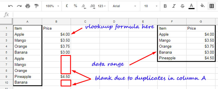
In the following example, I have search keys in the range A2:A10, which are fruit names, and the lookup table is in the range F2:G6, where the first column contains fruit names and the second column contains their prices.
Looking at the search keys, you can see that some fruits are repeated. I want a VLOOKUP formula in cell B2 that excludes duplicate search keys and returns results only for the first occurrence.
Exclude Duplicate Search Keys in VLOOKUP Using a Drag-Down Formula
As per the example above, you can use the following formula in cell B2 and drag it down:
=IF(
   COUNTIF($A$2:A2, A2)=1,
   VLOOKUP(A2, $F$2:$G$6, 2, FALSE),
)
How does this formula work?
The COUNTIF formula, COUNTIF($A$2:A2, A2), returns the running count of the search key as you drag it down. As you drag the formula down, the range becomes $A$2:A3, $A$2:A4, and so on, with the criterion becoming A3, A4, etc. The formula returns the count of the current item up to that row, which is the running occurrence.
The IF function evaluates whether the COUNTIF result is 1, and if it’s TRUE, it executes the VLOOKUP; otherwise, it returns a blank.
This is how you can exclude duplicate search keys in a VLOOKUP drag-down formula. Now, let’s see how to achieve the same result with a VLOOKUP array formula that expands down from B2.
Exclude Duplicate Search Keys in VLOOKUP Array Formula Result
The formula follows the same logic as above. The difference is that you should specify the search key range A2:A10 in the VLOOKUP instead of just A2. You’ll also need to replace the COUNTIF formula with a COUNTIFS formula. Additionally, the formula must be entered as an array formula.
Empty the range B2:B and insert the following formula in cell B2:
=ArrayFormula(
   IF(
      COUNTIFS(A2:A10, A2:A10, ROW(A2:A10), "<="&ROW(A2:A10))=1,
      VLOOKUP(A2:A10, F2:G6, 2, FALSE),
  )
)
Here’s how it works:
- The
COUNTIFS(A2:A10, A2:A10, ROW(A2:A10), "<="&ROW(A2:A10))part returns the running occurrence of the VLOOKUP search keys. - The IF function returns TRUE wherever the COUNTIFS result is 1 and executes the VLOOKUP array formula in those rows.
This is how we can exclude duplicate search keys in the VLOOKUP array result in Google Sheets.
Resources
- Using VLOOKUP to Find the Nth Occurrence in Google Sheets
- VLOOKUP with Multiple Criteria in Google Sheets: The Proper Way
- Retrieve Multiple Values Using VLOOKUP in Google Sheets
- VLOOKUP: Skip Blank Cells and Continue Search – Google Sheets
- VLOOKUP in Max Rows in Google Sheets
- IF and VLOOKUP Combination in Google Sheets
- Move Index Column If Blank in VLOOKUP in Google Sheets
- VLOOKUP Skips Hidden Rows in Google Sheets – Formula Example
- VLOOKUP Result Plus Next ‘n’ Rows in Google Sheets
- VLOOKUP Last Record in Each Group in Google Sheets
- How to Use VLOOKUP on Duplicates in Google Sheets
- How to Get Dynamic Search Column in VLOOKUP in Google Sheets
- Google Sheets – VLOOKUP Adjacent Cells


I am trying to use this with a question bank I have for google forms, but I am not putting in the right info to get it to work. Below is the Vlookup formula I am using, which pulls from another sheet with questions on it. Can you please help me fix this?
=vlookup(randbetween(1,max(questions!$A:$A)),questions!$A$2:$B,2,false)Could you please explain a bit more?