Combine product codes using comma, hyphen or a pipe symbol as the separator and lookup multiple rates or quantity in a flash. Yes! You can use such keyword combinations in Vlookup in Docs Sheets.
To use keyword combinations as the search keys in Vlookup, you can use the function Split with Vlookup. It’s a very simple to understand combination formula.
If this is something interesting to you, just read on to understand how to use combination keywords in Vlookup in Google Sheets.
Forming Combination Keywords to Use in Vlookup
I am not working in any manufacturing company or don’t even have my own product to sell. So I am not following inventory basics to form the product codes for our example.
Here I am just creating a few product codes using numbers and letters. So that I can make you understand how to form combination keywords.
It’s not necessary to use product codes to create combination keywords. You can just combine product names itself as the keyword combination.
What important is, it must be (whether its product codes or product names) in the first column in your Lookup table.
Sample Data:
| A | B | C | |
| 1 | Product Code | Qty. | Rate |
| 2 | KVP45 | 15 | $78.00 |
| 3 | KVP46 | 100 | $76.00 |
| 4 | KVP47 | 100 | $76.00 |
| 5 | KVP48 | 18 | $78.00 |
| 6 | KVP49 | 96 | $79.00 |
| 7 | KVP50 | 100 | $95.00 |
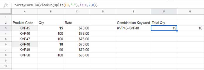
Here I can use the product codes “KVP45” and “KVP48” as the keyword combination “KVP45-KVP48” to use in Vlookup as the search key. You can form similar combinations from any other product codes in the list.
In this example, I have used a hyphen as the separator. Sometimes the product code or product name may already contain the hyphen. In such cases, either use the comma or pipe symbol as the separator. You feel free to combine more than two search keys (product codes or product names).
Suppose I want Lookup the Qty. of these two products (combined above) and total it. We can use Vlookup for that.
How to Use Keyword Combinations in Google Sheets Vlookup Formula
I am using the data in the above table and the combination product codes as the search keys in Vlookup.
Actually, the Keywords to use in Vlookup are “KVP45” and “KVP48” which are combined using a hyphen as the separator.
Of course in Vlookup, you can include multiple search keys. I have an earlier tutorial on that topic – How to Use Vlookup to Return An Array Result in Google Sheets. The same technique I am going to follow here.
We must first split the search keys using the Split function within Vlookup.
=split(E3,"-")Use the above Split formula as the search_key in Vlookup (vertical lookup which searches down the column # 1 in the range).
=VLOOKUP(search_key, range, index, [is_sorted])When using two or more search_keys, use the ArrayFormula function. Otherwise, Vlookup will only return the lookup value of the first search key.
=ARRAYFORMULA(VLOOKUP(search_keys, range, index, [is_sorted]))You May Like: Array Formula: How It Differs in Google Sheets and Excel.
The following formula is an example of the use of keyword combinations in Vlookup in Sheets.
=ArrayFormula(vlookup(split(E3,"-"),A3:C,2,0))
If you want to get the total of the Lookup values (Qty. here), wrap the Vlookup with the function Sum.
=ArrayFormula(sum(vlookup(split(E3,"-"),A3:C,2,0)))This will return the value 33 which is the total of the above Lookup values.
I always use the IFERROR function with Vlookup. This will be useful to avoid errors in case the search key is not available in Vlookup.
For example in the above formula, if any of the search keys are not available, the formula would return an error instead of returning the qty. of the available search key.
=ArrayFormula(sum(IFERROR(vlookup(split(E3,"-"),A3:C,2,0))))Conclusion
I have 35+ tutorial on this blog pertaining to Vlookup use. To read that search this blog using the search icon on the navigation bar.
If you don’t have enough time, at least check this one – Vlookup in Google Sheets – 10 Formula Variations, Tips, and Tricks.
Thanks for the stay. Enjoy!


