You may need different techniques to work effectively with VLOOKUP with comma-separated values in Google Sheets. Whether the search keys are comma-separated or the search column (the first column in the range) contains comma-separated values determines the approach.
This tutorial addresses both scenarios:
- VLOOKUP with Comma-Separated Values in the Search Column
- VLOOKUP with Comma-Separated Search Keys
1. VLOOKUP with Comma-Separated Values in the Search Column
Using the VLOOKUP function with a comma-separated value column is straightforward in Google Sheets. Here are two simple methods, with the second method introducing case sensitivity to the search.
Sample Data:
The sample data consists of comma-separated items in the first column and their total quantities in the second column. The range is B2:C. The search key (a product name) is in cell E2. Let’s see how to look up this product in B2:B and return the quantity of the first occurrence in the comma-separated list.
Option 1: Using the Asterisk Wildcard Character
Formula:
=IFNA(VLOOKUP("*"&E2&"*", B2:C, 2, FALSE))This formula will return 27 when the search key in cell E2 is “Product 11.” Let’s break it down.
Explanation:
- Search_key:
"*"&E2&"*"— Combines the search key with the asterisk wildcard on both ends for partial matches. - Range:
B2:C - Column index:
2 - Is_sorted:
FALSE— Ensures an exact match is required and handles unsorted ranges.
The IFNA function returns a blank instead of #N/A if the search key is not present.
To handle multiple search keys in the comma-separated list, use an array formula:
=ARRAYFORMULA(IFNA(VLOOKUP(IF(E2:E="",,"*"&E2:E&"*"), B2:C, 2, FALSE)))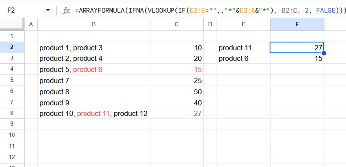
The IF(E2:E="",, "*" & E2:E & "*") part returns a blank if the search key is empty; otherwise, it adds wildcards (*) before and after the search key. This ensures that empty cells in the criteria range are ignored. Without this, the formula would use "**" as the search key and might return incorrect results.
Option 2: Using REGEXMATCH
The wildcard character method works well, but if you require case sensitivity, consider the REGEXMATCH approach.
Formula:
=IFNA(VLOOKUP(TRUE, HSTACK(ARRAYFORMULA(REGEXMATCH(B2:B, E2)), C2:C), 2, FALSE))This is a case-sensitive formula that handles a single search key in E2. Here’s how it works:
Explanation:
- Search_key:
TRUE(We use TRUE because the range contains TRUE or FALSE values in the first column, which are generated by the REGEXMATCH function below.) - Range:
HSTACK(ARRAYFORMULA(REGEXMATCH(B2:B, E2)), C2:C)— The REGEXMATCH function performs a case-sensitive partial match in columnB, and the result is combined with columnCusing HSTACK. - Column index:
2 - Is_sorted:
FALSE
A drawback of this approach is its inability to return array results. To handle multiple search keys, convert it into a custom lambda function and use it within the MAP function:
=ARRAYFORMULA(IF(E2:E="",,MAP(E2:E, LAMBDA(keys, IFNA(VLOOKUP(TRUE, HSTACK(REGEXMATCH(B2:B, keys), C2:C), 2, FALSE))))))- The
MAPfunction applies the LAMBDA function (LAMBDA(keys, IFNA(VLOOKUP(TRUE, HSTACK(REGEXMATCH(B2:B, keys), C2:C), 2, FALSE)))) to each row in the provided array (E2:E) and returns an array result. - The IF function ensures that the formula returns results only for non-empty cells in the search key range.
This formula is resource-intensive but effective for case-sensitive searches.
2. VLOOKUP with Comma-Separated Search Keys
VLOOKUP with comma-separated search keys is a different concept. Here, the search keys themselves are comma-separated, not the values in the search range.
Sample Data:
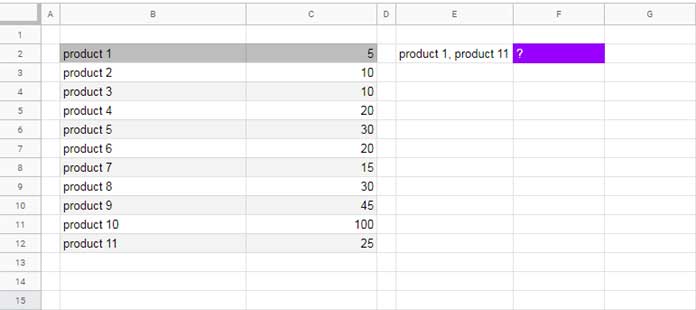
The data is in B2:C, and the comma-separated search keys are in cell E2.
Option 1: Case-Insensitive Formula
Formula:
=ARRAYFORMULA(IFNA(VLOOKUP(TRIM(SPLIT(E2, ",")), B2:C, 2, FALSE)))Explanation:
- Search_key:
TRIM(SPLIT(E2, ","))—Splits the search keys at the comma delimiter, and TRIM removes extra spaces. - Range:
B2:C - Column index:
2 - Is_sorted:
FALSE
The formula would return two values, 5 and 25, in two separate cells in the row. To combine the results into a single cell, use TEXTJOIN:
=TEXTJOIN(", ", TRUE, ARRAYFORMULA(IFNA(VLOOKUP(TRIM(SPLIT(E2, ",")), B2:C, 2, FALSE)))) // returns 5, 25To sum the results, use SUM:
=SUM(ARRAYFORMULA(IFNA(VLOOKUP(TRIM(SPLIT(E2, ",")), B2:C, 2, FALSE)))) // returns 30If the search keys are in multiple rows (e.g., E2:E), adapt the formula:
=ARRAYFORMULA(IFERROR(VLOOKUP(TRIM(SPLIT(E2:E, ",")), B2:C, 2, FALSE)))The results will be in multiple rows, but not combined or totaled row by row.
For expanded combined results, use the MAP function:
=IFERROR(MAP(E2:E, LAMBDA(val, TEXTJOIN(", ", TRUE, ARRAYFORMULA(VLOOKUP(TRIM(SPLIT(val, ",")), B2:C, 2, FALSE))))))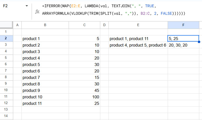
You can replace TEXTJOIN(", ", TRUE, ...) with SUM(...) to total the results in each row, instead of combining them.
Option 2: Case-Sensitive Formula
For case-sensitive searches, use the FILTER function.
You might wonder why I don’t recommend VLOOKUP — this is because combining REGEXMATCH doesn’t work well in this case. Since multiple search keys are returned in the SPLIT function, REGEXMATCH will match all of them and return an array of TRUE or FALSE values. If you use TRUE as the search key in VLOOKUP, it will only return the value corresponding to the first TRUE.
Therefore, I suggest using the FILTER function, which can filter all values corresponding to the TRUE values. Learn more here: Comma-Separated Values as Criteria in Filter Function in Google Sheets.
Wrap-Up: VLOOKUP with Comma-Separated Values
We have explored two approaches for using VLOOKUP with comma-separated values in Google Sheets. In the first approach, the first column in the range contains the comma-separated values, while in the second approach, the search keys are comma-separated.
You can use array formulas in both approaches to expand results. Additionally, I’ve included ways to add case-sensitivity to these formulas.
I hope you find these methods useful. Below are some additional resources.
Resources
- VLOOKUP and Combine Values in Google Sheets
- Replace Multiple Comma-Separated Values in Google Sheets
- How to Count Comma-Separated Words in a Cell in Google Sheets
- Sum, Count, Cumulative Sum Comma-Separated Values in Google Sheets
- Extract Unique Values from a Comma-Separated List in Google Sheets
- Split Comma-Separated Values in a Multi-Column Table in Google Sheets
- How to Remove Duplicates from Comma-Delimited Strings in Google Sheets
- How to Compare Comma-Separated Values in Google Sheets


The Vlookup part of the non-sum formula gives an error as it’s not able to find the first value from the split. Did anything change?
Hi, Pritesh,
It works in my test. Make sure that the cell range F2:2 is empty.
Additional Tip: This will remove blanks in the result.
=transpose(sort(transpose(IFNA(vlookup(trim(split(E2,",")),B2:C12,2,0)))))Hi Prashanth,
How can we do the Vlookup and receive a sum of multiple values when the search key being used is delimited with multiple values (“red|blue|green”). The example above only seems to sum one value and not an array of values.
Hi, Mirko,
I think I have already provided the formula in the tutorial.
If that is not helpful, please share your sample data. You can share the link via “Reply”.
Hi,
How can I get Sum if I have multiple columns to look up and sum values?
In the above example, you have shown the Lookup index as 2. But I have Lookup index as a range from column 2 to 4 and product 1 and product 11 separated with a comma.
I tried;
=arrayformula(sum(VLOOKUP(split(K4,"/"),A2:E14,arrayformula(COLUMN(B2:D2)),0)))But it is not working. Can you please help me?
Hi, Harshida,
Your formula is not in line with my instructions. Here are a few of the issues in your formula.
1. Missing the TRIM() function.
2. Instead of
column(B2:D2)you must usetranspose(column(B2:D2))orrow(A2:A4).Also, the separator is not a comma but a forward slash.
Here is the Vlookup formula (with comma-separated search keys) after the above modifications.
=ArrayFormula(SUM(IFNA(vlookup(trim(split(K4,"/")),A2:E14,row(A2:A4),0))))