We can use the VLOOKUP function to look up a value and return the sum of values from matching rows in Google Sheets.

This is a very useful scenario. For example, you can look up a student’s name in column A and return their total marks from columns B, C, D, E, or any other chosen columns.

If the student’s name appears in multiple rows, one row for midterm marks and another for finals, you can get the totals altogether. Here is how to do it using VLOOKUP and alternative solutions.

Using VLOOKUP to Sum Values in a Row

In the following example, we have student names in column A, exam types in column B, and their marks in Maths, Science, and English in columns C to E. Row 1 (A1:E1) contains the field labels.

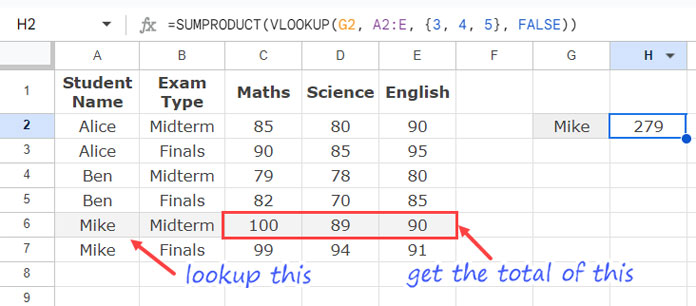
The following VLOOKUP formula will look up the name “Mike” entered in cell G2 in the first column of the range A2:E and return the total of his marks in Maths, Science, and English from the found row within the range (third, fourth, and fifth columns).

=SUMPRODUCT(VLOOKUP(G2, A2:E, {3, 4, 5}, FALSE))

This is the basic example of VLOOKUP to sum values in a row.

Formula Breakdown:

The formula has two parts: the VLOOKUP part and the SUMPRODUCT part.

VLOOKUP Part: VLOOKUP(G2, A2:E, {3, 4, 5}, FALSE)

If you enter this part as an array formula like =ARRAYFORMULA(VLOOKUP(G2, A2:E, {3, 4, 5}, FALSE)), it will return the marks of “Mike” in Maths, Science, and English in three columns. However, we haven’t used the ARRAYFORMULA since we use SUMPRODUCT. I’ll explain why in the next section.

The formula follows the syntax:

VLOOKUP(search_key, range, index, [is_sorted])

Where:

• search_key: G2 (the cell containing the lookup value, which is “Mike” in this case).
• range: A2:E (the lookup range for the search key where the formula will look up the search key in the first column, i.e., A2:A).
• index: {3, 4, 5} (the column numbers in the range from which to extract the values).
• is_sorted: FALSE (means the range is not sorted and looks up the exact match of the search_key).

SUMPRODUCT Part:

The function SUMPRODUCT returns the sum of the products of two elements in two arrays. If you specify only one array, as with the VLOOKUP result here, it will simply return the sum.

Syntax:

SUMPRODUCT(array1, [array2, …])

However, we do not need to use ARRAYFORMULA with SUMPRODUCT, as SUMPRODUCT inherently works as an array function.

Using VLOOKUP to Sum Values in Multiple Rows

VLOOKUP and other lookup functions are designed to return values matching the first occurrence of the search key (from the top or bottom depending on the function).

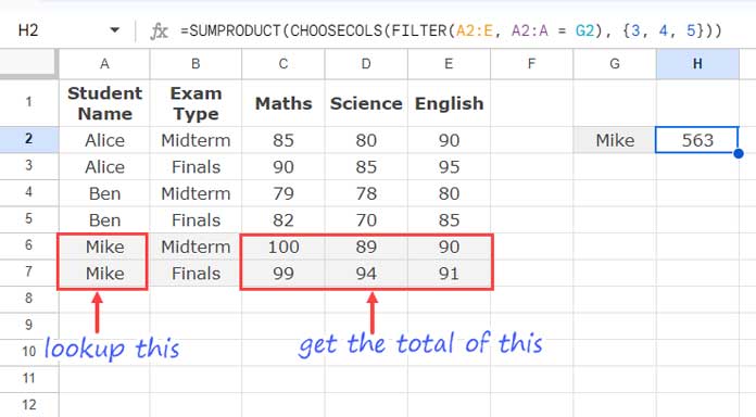
Since VLOOKUP can only return the value from the first occurrence, to sum values across multiple rows, we need to use an alternative formula:

=SUMPRODUCT(CHOOSECOLS(FILTER(A2:E, A2:A = G2), {3, 4, 5}))

This formula has three parts: FILTER, CHOOSECOLS, and SUMPRODUCT.

• FILTER: This function filters the range A2:E based on the condition that values in A2:A are equal to the lookup value in cell G2. It returns only the rows where the condition is TRUE.
• CHOOSECOLS: This function selects the specified columns (3, 4, 5) from the filtered result.
• SUMPRODUCT: This function sums the values from the selected columns.

This approach provides a workaround for summing values from multiple rows that match the search key, which VLOOKUP cannot handle.

This is the best workaround when you want to VLOOKUP and sum values from multiple rows.

How to Sum Marks for Each Student Individually

In the above examples, we calculated the total marks for a single student. What if we need to do the same for more than one student?

In that case, instead of summarizing based on individual search keys, you can summarize the marks of students using the QUERY function as follows:

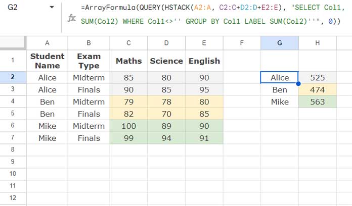
=ArrayFormula(QUERY(HSTACK(A2:A, C2:C+D2:D+E2:E), "SELECT Col1, SUM(Col2) WHERE Col1<>'' GROUP BY Col1 LABEL SUM(Col2)''", 0))

Where:

• A2:A is the column to group by, i.e., the student names column (Col1).
• C2:C+D2:D+E2:E represents the total marks (Col2).

The formula selects Col1 and sums Col2, grouping by Col1. Additionally, it removes blank rows and the label from the top of the sum column.

Resources

• Combined Use of SUMIF with VLOOKUP in Google Sheets
• Using VLOOKUP to Find the Nth Occurrence in Google Sheets
• VLOOKUP with Multiple Criteria in Google Sheets: The Proper Way
• Retrieve Multiple Values Using VLOOKUP in Google Sheets
• VLOOKUP Result Plus Next ‘n’ Rows in Google Sheets
• Google Sheets – VLOOKUP Adjacent Cells