How do you VLOOKUP adjacent cells in Google Sheets? Before answering that, let’s first clarify what we mean by adjacent cells.
If you consider the search key, adjacent cells refer to the ones immediately to the right, top, or bottom of the matched value within the range.
But when we talk about the output of a VLOOKUP, adjacent cells can be any cells around the returned value—left, right, top, or bottom. While it’s easy to get the left or right value using the index number, fetching the top or bottom value isn’t possible through index adjustment alone.
That’s where a combination of VLOOKUP and OFFSET comes in handy to retrieve adjacent cell values in Google Sheets—without modifying the index number.
Cheque Received from Customers – Sample Data
Let’s work with this sample dataset in the range A1:E5.
| Customer | Cheque # | Bank | Date | Amount |
|---|---|---|---|---|
| Customer A | 912775 | Bank I | 15/12/19 | 6500.00 |
| Customer B | 271057 | Bank II | 18/12/19 | 8000.00 |
| Customer C | 271058 | Bank II | 18/12/19 | 25000.00 |
| Customer D | 912776 | Bank I | 15/12/19 | 4050.00 |
Assume you’ve received cheque payments from your customers and recorded them in Google Sheets in the order they were received.
We’ll now explore how to:
- Use a customer name to find the cheque number next to it.
- Retrieve the cheque received just before or after.
- Identify which customer made the prior or next payment.
This information can be useful for tracking payment sequence, spotting duplicates, or understanding customer behavior based on payment timelines.
VLOOKUP Adjacent Cells (Relative to the Result) in Google Sheets
1. Return Value Just Above the VLOOKUP Result
Let’s say the search key is "Customer C" and we’re using Column B (Cheque #) as the return column.
Basic VLOOKUP:
=VLOOKUP("Customer C", A2:E, 2, FALSE)To get the value just above the cheque number:
=OFFSET(VLOOKUP("Customer C", A2:E, 2, FALSE), -1, 0)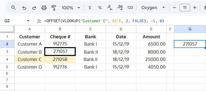
2. Return Value Just Below the VLOOKUP Result
To fetch the cheque received immediately after the one from Customer C:
=OFFSET(VLOOKUP("Customer C", A2:E, 2, FALSE), 1, 0)3. Return Value to the Left of the VLOOKUP Result
If you want to get the value from the left of the VLOOKUP return cell:
=OFFSET(VLOOKUP("Customer C", A2:E, 2, FALSE), 0, -1)4. Return Value to the Right of the VLOOKUP Result
To get the value to the right of the returned cheque number:
=OFFSET(VLOOKUP("Customer C", A2:E, 2, FALSE), 0, 1)VLOOKUP Adjacent Cells (Relative to the Search Key) in Google Sheets
This one’s a bit different. If you run a basic VLOOKUP like:
=VLOOKUP("Customer C", A2:E, 1, FALSE)…it will simply return the search key, “Customer C.” But that return value can’t be used with OFFSET to reference nearby cells directly because VLOOKUP doesn’t return a cell reference—only the value.
So, instead, use a VLOOKUP that returns a different column (like Column B), and OFFSET relative to that cell.
Value Above the Search Key (Customer Name)
To get the customer who paid just before Customer C:
=OFFSET(VLOOKUP("Customer C", A2:E, 2, FALSE), -1, -1)Value Below the Search Key
To get the next customer after Customer C:
=OFFSET(VLOOKUP("Customer C", A2:E, 2, FALSE), 1, -1)These OFFSET + VLOOKUP combinations help you reference cells relative to the search key, even when it’s in the first column.
Conclusion
As shown in the examples above, you can combine OFFSET with VLOOKUP to fetch adjacent cells in Google Sheets. The key is understanding where you’re anchoring your lookup—from the return column or from the search key column.
When using VLOOKUP to access adjacent cells, be especially careful if the search key lies in the first column—OFFSET won’t work directly on the value returned by index 1. You’ll need to offset from another column’s return instead.


