This tutorial explains how to use VLOOKUP and combine values in Google Sheets using both array and non-array formulas. Along the way, you’ll uncover some of the most useful tips, ideas, and tricks for working with Google Sheets.
If there are multiple occurrences of a lookup value (search_key) in the lookup column (the first column in the VLOOKUP range), the VLOOKUP function in Google Sheets generally returns only the value corresponding to the first occurrence.
This behavior might not be ideal for all situations. Fortunately, Google Sheets offers functions like FILTER and QUERY to solve this challenge.
VLOOKUP and Combine Values in Google Sheets – Non-Array Alternative
Here’s an example of how to use VLOOKUP and concatenate values:
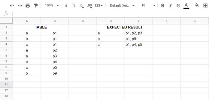
If we use the following ArrayFormula VLOOKUP in cell E2, we will only get the value “p1” in cells E2, E3, and E4. These are the values corresponding to the first occurrences of the search keys “a”, “b”, and “c”:
=ArrayFormula(VLOOKUP(D2:D4, A2:B9, 2, 0))However, using the following FILTER + UNIQUE + TEXTJOIN formula in cell E2, we get the correct result, i.e., “p1, p2, p3”, for the first search key, which is “a”:
=TEXTJOIN(", ", TRUE, UNIQUE(FILTER($B$2:$B, $A$2:$A = D2)))For the search keys “b” and “c”, you would need to use the above formula in cell E2, then drag it down until cell E4.
Explanation of the Formula:
- The FILTER function filters the range
B2:BwhereverA2:Amatches the key inD2. - The UNIQUE function returns unique values (optional).
- The TEXTJOIN function combines those values, leaving a comma as the delimiter.
This is the non-array alternative for VLOOKUP and combining values in Google Sheets.
VLOOKUP and Combine Values in Google Sheets – Array Formula Alternatives
There are two different approaches for using an array formula.
You can transform the above FILTER-based formula into an unnamed lambda function and apply it to each element in the search key range (D2:D4) using a lambda helper function.
Alternatively, you can use a QUERY workaround as an alternative to VLOOKUP and combine values.
Approach 1: Using the LAMBDA Function
We can create a custom function based on the FILTER formula above as follows:
=LAMBDA(search_key, TEXTJOIN(", ", TRUE, UNIQUE(FILTER($B$2:$B, $A$2:$A = search_key))))You can test it by specifying the function call with D2, like this:
=LAMBDA(search_key, TEXTJOIN(", ", TRUE, UNIQUE(FILTER($B$2:$B, $A$2:$A = search_key))))(D2)This is equivalent to the FILTER formula above. Now, we can convert it into an array formula by specifying the lambda function within the MAP function, which iterates over each element in the array D2:D4 and returns an array result.
The syntax for the MAP function is:
=MAP(array1, [array2, …], lambda)Where array1 is D2:D4, the search key range, and lambda is the above lambda function without the function call.
=MAP(D2:D4, LAMBDA(search_key, TEXTJOIN(", ", TRUE, UNIQUE(FILTER($B$2:$B, $A$2:$A = search_key)))))In our example, you can use this formula in cell E2 after clearing the range E2:E4.
Approach 2: Using a QUERY Workaround
In this approach, I will explain the process step by step so you can understand how the formula develops and learn new techniques.
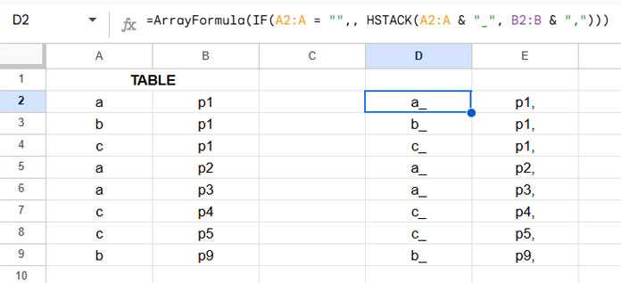
Step 1:
=ArrayFormula(IF(A2:A = "",, HSTACK(A2:A & "_", B2:B & ",")))This array formula adds an underscore at the end of the values in A2:A and a comma at the end of the values in B2:B if A2:A is not empty.
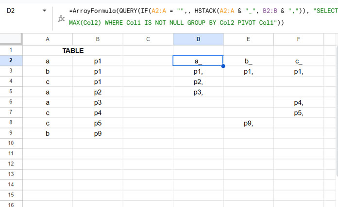
Step 2:
=ArrayFormula(QUERY(IF(A2:A = "",, HSTACK(A2:A & "_", B2:B & ",")), "SELECT MAX(Col2) WHERE Col1 IS NOT NULL GROUP BY Col2 PIVOT Col1"))- SELECT MAX(Col2) WHERE Col1 IS NOT NULL: Returns the maximum value in column 2 (i.e.,
p9,). - SELECT MAX(Col2) WHERE Col1 IS NOT NULL GROUP BY Col2: Returns the unique values in column 2 (i.e., {
p1,,p2,,p3,,p4,,p5,,p9,}). - SELECT MAX(Col2) WHERE Col1 IS NOT NULL GROUP BY Col2 PIVOT Col1: Pivots the unique values in
Col1(e.g.,a_,b_,c_) into column headers and places all the corresponding unique values from column 2 under the relevant columns.
Step 3:
=ArrayFormula(TRANSPOSE(QUERY(QUERY(IF(A2:A = "",, HSTACK(A2:A & "_", B2:B & ",")), "SELECT MAX(Col2) WHERE Col1 IS NOT NULL GROUP BY Col2 PIVOT Col1"),, 9^9)))The QUERY function combines values in each column into a single row, considering them all as part of the headers. The TRANSPOSE function changes the orientation of the result.
| a_ p1, p2, p3, |
| b_ p1, p9, |
| c_ p1, p4, p5, |
Step 4:
=ARRAYFORMULA(REGEXREPLACE(TRIM(SPLIT(TRANSPOSE(QUERY(QUERY(IF(A2:A="",, HSTACK(A2:A&"_", B2:B&",")),"SELECT MAX(Col2) WHERE Col1 IS NOT NULL GROUP BY Col2 PIVOT Col1"),, 9^9)), "_")), "^,\s|,$", ""))Finally, we split the text using the underscore delimiter, which is an alternative to VLOOKUP for combining values in Google Sheets. During this process, we use functions like TRIM and REGEXREPLACE to remove extra spaces and delimiters from the start and end of the combined string.


