Offset VLOOKUP Results to the Correct Header Columns in Google Sheets

If you’ve ever needed to spread data across date-based columns in Google Sheets — for example, to return a quantity based on multiple criteria and place it under the matching header (like a PO date) — this tutorial is for you.

We’ll show how to use VLOOKUP (or XLOOKUP) to match a combination of P.O. No. and Item, retrieve the Qty, and then offset the result to the correct column using the header date.

By the end, you’ll learn how to transform tall data into a wide table using a single array formula — perfect for dashboards, reports, or pivot-style summaries in Google Sheets.

Table of Contents

Sample Data and Lookup Setup

Let’s start with a sample dataset located in the Item sheet tab. This is our lookup table:

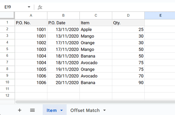
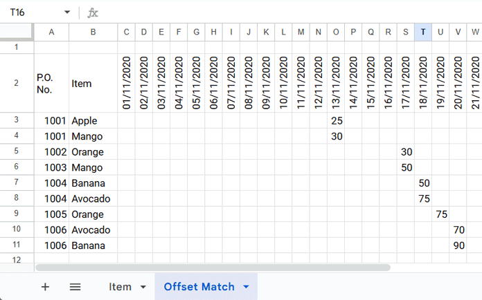
Sample purchase order data with P.O. No., P.O. Date, Item, and Qty columns in Google Sheets

In a second table, we want to populate quantities under date headers, based on matching P.O. No. and Item.

Here’s what that looks like:

Offset VLOOKUP results showing quantities placed under matching date headers in Google Sheets

Goal: Offset VLOOKUP Results to Matching Headers

We want to:

Search for Qty using multiple criteria (P.O. No. + Item).
Find the matching date (P.O. Date).
Place Qty under the correct date column (offset to the header).

Step-by-Step Guide

Step 1: Lookup the Quantity (Value to Offset)

Use VLOOKUP where the search key is a combination of P.O. No. and Item. The lookup table is also adjusted accordingly by combining P.O. No. and Item, and stacking it with the Qty using HSTACK.

=ArrayFormula(
  VLOOKUP(
    A3:A & " " & B3:B,
    HSTACK(Item!A2:A & " " & Item!C2:C, Item!D2:D),
    2,
    FALSE
  )
)

Result:

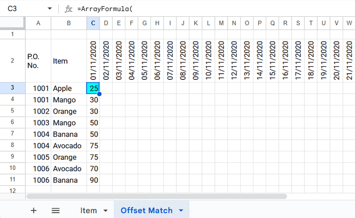
VLOOKUP formula output showing quantity values based on combined P.O. No. and Item in Google Sheets

Explanation:

A3:A & ” ” & B3:B combines P.O. No. and Item (multiple criteria).
HSTACK(...) creates a two-column lookup range: criteria + Qty.
2 is the index to return Qty.

Note: You can test this formula separately in the result sheet to see the intermediate output. However, this isn’t required, as we’ll combine all steps into a single formula later.

Step 2: Lookup the Date (To Match Header)

Now use a similar formula to lookup the P.O. Date:

=ArrayFormula(
  VLOOKUP(
    A3:A & " " & B3:B,
    HSTACK(Item!A2:A & " " & Item!C2:C, Item!B2:B),
    2,
    FALSE
  )
)

Result:

This returns the date associated with each row, which will be compared to the date headers in your output table.
(The result will be date values that can be formatted as dates, but formatting isn’t necessary here since they are used within another formula, not displayed directly in a cell.)

Step 3: Offset the Quantity to the Matching Header Column

Combine steps 1 and 2 into one formula that places the value under the matching date column:

=ArrayFormula(
  IF(
    VLOOKUP(A3:A & " " & B3:B, HSTACK(Item!A2:A & " " & Item!C2:C, Item!B2:B), 2, FALSE) = C2:AF2,
    VLOOKUP(A3:A & " " & B3:B, HSTACK(Item!A2:A & " " & Item!C2:C, Item!D2:D), 2, FALSE),
    ""
  )
)

C2:AF2 is the row with date headers.
The formula compares each row’s lookup date to each column header.
If matched, it returns the Qty in that cell. Otherwise, it shows a blank.

Result: You now have quantities auto-filled in the correct date columns — no manual copying or filtering needed.

Bonus: Use XLOOKUP for Cleaner Formula

With XLOOKUP, the formula becomes simpler and more readable:

=ArrayFormula(
  IF(
    XLOOKUP(A3:A & " " & B3:B, Item!A2:A & " " & Item!C2:C, Item!B2:B) = C2:AF2,
    XLOOKUP(A3:A & " " & B3:B, Item!A2:A & " " & Item!C2:C, Item!D2:D),
    ""
  )
)

Why XLOOKUP is Better Here:

You don’t need to HSTACK ranges.
You can directly define the lookup range and return range.
Easier to read and maintain.

Final Output: Tall to Wide Transformation

You’ve now transformed your row-wise (tall) purchase order data into a column-wise (wide) matrix, where each quantity is placed under the corresponding date — automatically.

This method is especially useful for:

Daily reports
Stock movement logs
Invoice tracking
Attendance data, etc.

Copy Sample Sheet

👉 Click here to make a copy of the sample Google Sheet