Whether you’re just getting started or have used VLOOKUP hundreds of times, chances are you’ve run into a few frustrating errors. Don’t worry — you’re not alone. In this guide, I’ll walk you through the most common errors in VLOOKUP in Google Sheets, why they happen, and how to fix them quickly.
To keep things simple, I’ve grouped these into two main types:
- Syntax errors — These trigger actual error messages like
#N/A!,#REF!,#VALUE!,#ERROR!, and#NAME?. - Accidental mistakes — These won’t trigger an error message but might give you the wrong result, which is arguably worse.
Let’s tackle each one — with clear examples and fixes.
Google Sheets VLOOKUP Error Quick Diagnostic Guide
If your VLOOKUP formula is returning an error in Google Sheets, it is usually caused by a range mismatch, formatting issue, or a minor spelling typo. Use this quick diagnostic table to identify your specific error code, understand its root cause, and apply the immediate fix:
| Error | Root Cause | Quick Fix |
|---|---|---|
#N/A | Search key not found | Use IFNA or verify the lookup value |
#VALUE! | Invalid argument | Check argument order and column index |
#REF! | Invalid range or column index outside lookup range | Correct the range or index |
#ERROR! | Formula parse error | Check syntax, argument separators (, or ;), quotes, and sheet references. |
#NAME? | Misspelled function or invalid named range | Correct spelling or named range |
Syntax-Based VLOOKUP Errors in Google Sheets
These are the typical VLOOKUP errors that throw up #N/A, #REF!, #VALUE!, and other error messages when your formula syntax goes wrong.
#N/A Error: Search Key Not Found
Tooltip: Did not find value ‘Student 6’ in VLOOKUP evaluation.
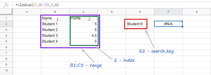
This is hands down the most common error in VLOOKUP. It simply means: “I looked, but I didn’t find what you asked for.”
Example:
=VLOOKUP(E2, B1:C5, 2, FALSE)If the value in E2 (“Student 6”) isn’t in the first column of the range (B1:B5), VLOOKUP gives you the dreaded #N/A!.
How to Fix the #N/A Error:
You’ve got a few options depending on what you want to show instead of the error:
- Return a blank:
=IFNA(VLOOKUP(E2, B1:C5, 2, FALSE)) - Return a custom message:
=IFNA(VLOOKUP(E2, B1:C5, 2, FALSE), "Student not found") - Return 0 instead:
=IFNA(VLOOKUP(E2, B1:C5, 2, FALSE), 0)
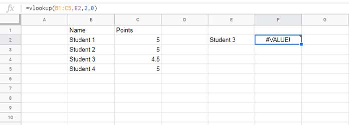
#VALUE! Error — Invalid Arguments
The #VALUE! error usually means there’s a problem with how you’ve entered the arguments in your VLOOKUP formula.
Common Causes of the #VALUE! Error:
- Wrong order of arguments:
=VLOOKUP(B1:C5, E2, 2, FALSE)
❌ Here, you’re putting the range first and the search key second — that won’t work.
✅ Correct it like this:=VLOOKUP(E2, B1:C5, 2, FALSE) - Using text instead of a column number:
=VLOOKUP(E2, B1:C5, "Points", FALSE)
The third argument (column index) should be a number — not a label. So use2instead of"Points". (Only database functions like DGET allow field labels — VLOOKUP doesn’t.) - Index is 0 (or less than 1):
=VLOOKUP(E2, B1:C5, 0, FALSE)
VLOOKUP columns start from 1, not 0 — so using 0 triggers this error.
#REF! Error — Invalid Reference
You’ll see #REF! when VLOOKUP points to a range that no longer exists.
Example:
=VLOOKUP(C2, #REF!, 2, FALSE)Maybe you deleted the original range, or the formula refers to cells that never existed — like using an invalid sheet name in the range (e.g., Sales!A1:C when the actual sheet is named SalesData).
Column Index Out of Bounds:
VLOOKUP(E2, B1:C5, 3, FALSE)If your range only has 2 columns but you enter 3 as the index. VLOOKUP can’t return a column that doesn’t exist in the range.
#ERROR! Error — Formula Parse Error
This error usually pops up when there’s something Google Sheets can’t interpret — like missing quotes, invalid references, or broken syntax.
Common Scenarios:
Unquoted sheet name with spaces:
=VLOOKUP("Apple", Sales Report!A1:B, 2, FALSE)❌ This causes a formula parse error.
✅ Fix it by adding single quotes:
=VLOOKUP("Apple", 'Sales Report'!A1:B, 2, FALSE)Invalid structured table reference:
=VLOOKUP("Ben", Table2[#ALL], 2, FALSE)If Table2 doesn’t exist (or isn’t created via Insert > Table), this will break with an error.
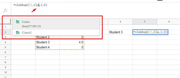
#NAME? Error — Misspelled Function or Named Range
This error often pops up because of:
- A typo in the function name:
=VLOOOKUP(E2, B1:C5, 2, FALSE) - Using a named range that doesn’t exist:
=VLOOKUP(E2, Classs, 2, FALSE) - Accidentally using a name instead of a column index:
=VLOOKUP(E2, B1:C5, Points, FALSE)
Pro Tip:
If you’re using Named Ranges, Google Sheets will auto-suggest them as you type. Just pick from the dropdown — that way, no spelling errors.
Common VLOOKUP Mistakes That Return Incorrect Results or Cause Errors
Now for the sneaky stuff — when your formula doesn‘t throw an error but still gives you the wrong result.
Extra Spaces
Spaces at the start or end of a value are invisible — but deadly in lookups.
Example:
Even this tiny space causes a mismatch:
=VLOOKUP("Student 3 ", B1:C5, 2, FALSE)In this case, there’s an accidental space after “Student 3” — and VLOOKUP won’t find a match.
Fix:
Make sure the search_key doesn’t include any extra spaces. A simple typo like that can return #N/A.
You can clean up your data in two ways:
- Manual option:
Select the column → go to Data → Data clean-up → Trim whitespace - Formula-based fix:
Use TRIM insideVLOOKUPto clean the lookup range:=ARRAYFORMULA(VLOOKUP(E2, TRIM(B1:C5), 2, FALSE))
And if the issue is on the search_key side (like in "Student 3 "), you can also wrap that with TRIM():
=VLOOKUP(TRIM(E2), B1:C5, 2, FALSE)Data Type Mismatch (Text, Number, or Date)
If your search key is a number but the column is formatted as text, VLOOKUP might return #N/A! — even if the numbers look the same.
Example Fixes:
- Ensure the first column in your range is formatted as Number, not Text.
- For dates, both the search key and the lookup column should contain real date values rather than one being a text string and the other a real date. This issue commonly occurs when you enter a date in a format that doesn’t match your Google Sheets locale, causing it to be stored as text instead of a date.
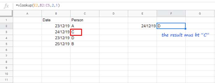
Incorrect Match Type (is_sorted)
This is a big one.
If you forget to specify the fourth argument in VLOOKUP (is_sorted), Google Sheets assumes it’s TRUE — which means “approximate match”.
Result:
You might get a wrong result that looks right — and never realize it.
How to Fix It:
Unless you know what you’re doing, always set it to FALSE:
=VLOOKUP(E2, B1:C5, 2, FALSE)Or, if you do want an approximate match, make sure the first column of the lookup range is sorted in ascending order.
Advanced Pro Tip: Isolating Source Errors Without Hiding Missing Keys
While IFNA is great for catching missing search keys, what happens if your search key is found, but the value you are retrieving contains a broken error (like #DIV/0!) that you want to replace with a clean warning message?
If you use IFERROR on the outside, you run into the “sledgehammer” problem we discussed above. But you can elegantly solve this by using LET and nesting an IFERROR directly inside your lookup array:
=LET(vl, VLOOKUP(E2, IFERROR(B1:C5, "Source Data Error"), 2, FALSE), IFNA(vl, "Not Found"))How This Formula Works:
- The Inner Shield:
IFERROR(B1:C5, "Source Data Error")catches errors inside your raw dataset before VLOOKUP even runs. If a cell is broken, it safely becomes a readable text string. - The Clean Return:
LET(vl, ...)holds that lookup result cleanly in memory. - The Outer Filter:
IFNA(vl, "Not Found")triggers only if the lookup key inE2completely missing from column A.
This gives you total control: you get a clean "Not Found" for missing keys, a custom "Source Data Error" for broken data cells, and actual formula typos (like an out-of-bounds index) will still break visibly so you can debug them!
Conclusion
That wraps up the most common errors in VLOOKUP in Google Sheets — both the ones that throw errors and the ones that sneak past without you noticing.
Get these right, and your formulas will become far more reliable (and less stressful to debug!).


