This tutorial will guide you on how to effectively use VLOOKUP on duplicates in Google Sheets.

When the search column (the first column in your data range) contains duplicates, using VLOOKUP in its default form will only return the value of the first match.

Let’s examine this with an example where the search key is in cell D2, and the data range is A2:B.

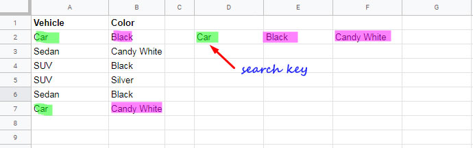
If you use the standard VLOOKUP formula as shown below, it will only return “Black” (the value from the second column of the first occurrence of the search key):

=VLOOKUP(D2, $A$2:$B, 2, FALSE)

In this case, the search key “Car” appears twice in the first column. If you want to retrieve values from the second column corresponding to both occurrences, you need alternative methods.

Using VLOOKUP on Duplicate Values in Google Sheets

If the VLOOKUP search column contains duplicates, the default function searches for the first occurrence of the search key and returns its corresponding value. To handle duplicates, you have two options:

1. Retrieve all duplicate values from the first column and their corresponding values from the second column.
2. Return values from specific duplicate occurrences (e.g., 1st, 2nd, etc.) from the first column.

In this tutorial, we will focus on the first option—how to use VLOOKUP to handle all duplicates. For retrieving specific occurrences, refer to VLOOKUP to Find Nth Occurrence in Google Sheets.

There are two primary methods:

1. Using the FILTER Function
2. Using VLOOKUP with an Array Formula

Using the FILTER Function as an Alternative to VLOOKUP

To get started, use the sample data mentioned earlier (A2:B) and apply the following FILTER formula:

=FILTER($B$2:$B, $A$2:$A=D2)

This formula filters column B based on rows where column A equals the search key “Car.” The output will include multiple rows. To display the results in a single row, wrap the formula with TRANSPOSE:

=TRANSPOSE(FILTER($B$2:$B, $A$2:$A=D2))

Place this formula in cell E2. To repeat the lookup for additional search keys, drag the fill handle down.

For a more efficient solution, you can use a custom LAMBDA function with the MAP helper function:

=MAP(D2:D5, LAMBDA(search_key, TRANSPOSE(FILTER($B$2:$B, $A$2:$A=search_key))))

This formula applies the FILTER logic to each search key in the range D2:D5. It’s a scalable way to perform VLOOKUP on duplicates with multiple search keys.

Using VLOOKUP on Duplicates with an Array Formula

If you need to perform VLOOKUP on duplicates for large datasets, the FILTER method may slow down your sheet. In such cases, you can use an array formula as an alternative.

Consider the following steps:

Create a pivot-like structure where duplicate values in the first column are merged, and their corresponding values occupy separate columns. Here’s how:

=ARRAYFORMULA(QUERY(QUERY({A2:B, COUNTIFS(A2:A, A2:A, ROW(A2:A), "<="&ROW(A2:A))},
"SELECT Col1, MAX(Col2) WHERE Col1 IS NOT NULL GROUP BY Col1 PIVOT Col3"),
"SELECT * OFFSET 1", 0))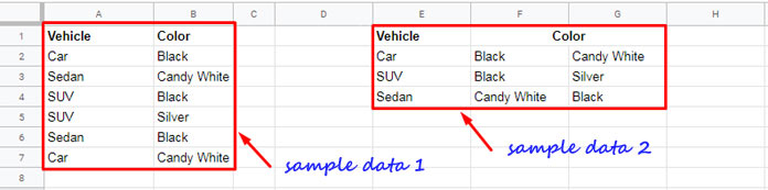

This formula creates a structured table where each unique key appears once, with its corresponding values arranged in separate columns.

Use this table as the range in your VLOOKUP formula:

=ARRAYFORMULA(IFERROR(VLOOKUP(D2:D5, QUERY(QUERY({A2:B, COUNTIFS(A2:A, A2:A, ROW(A2:A), "<="&ROW(A2:A))},
"SELECT Col1, MAX(Col2) WHERE Col1 IS NOT NULL GROUP BY Col1 PIVOT Col3"),
"SELECT * OFFSET 1", 0), {2,3,4,5}, FALSE)))

This formula retrieves all values corresponding to duplicates for each search key in D2:D5.

Note that {2,3,4,5} specifies the index numbers in VLOOKUP to return values from the 2nd to the 5th columns. The first column is omitted because it is the search key column. You can modify this array to include more columns if needed, such as {2,3,4,5,6,7,8,9,10}.

Conclusion

That’s it! You’ve learned two effective methods to handle duplicates using VLOOKUP in Google Sheets. Depending on your data size and requirements, you can choose either the FILTER method or the array formula.

Enjoy working with your data, and check out these additional resources:

• VLOOKUP: Skip Blank Cells and Continue Search – Google Sheets
• Exclude Duplicate Keys in VLOOKUP Array Result in Google Sheets
• VLOOKUP Skips Hidden Rows in Google Sheets – Formula Example
• VLOOKUP Result Plus Next ‘n’ Rows in Google Sheets
• VLOOKUP from Bottom to Top in Google Sheets
• Using Keyword Combinations in VLOOKUP in Google Sheets
• How to Get Dynamic Search Column in VLOOKUP in Google Sheets
• Using VLOOKUP to Sum Multiple Rows in Google Sheets
• Google Sheets – VLOOKUP Adjacent Cells
• VLOOKUP and Offset Multiple Criteria in Google Sheets (Array Formula)
• Filter VLOOKUP Result Columns in Google Sheets (Formula Examples)
• VLOOKUP on Every Other Column in Google Sheets