We need a universal solution, not specific to one function, to remove blank cells from the bottom of the ARRAYFORMULA output in Google Sheets.
Many functions return multiple rows when used with ARRAYFORMULA, such as VLOOKUP, XLOOKUP, SUMPRODUCT, SUMIF, COUNTIF, etc.
Therefore, you may require a common solution to address the issue of blank rows at the bottom of the result. These blank cells may prevent you from entering values in rows below the result.
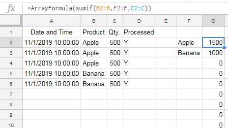
In the following example, the SUMIF formula in cell G2 uses the criteria range F2:F.
=ArrayFormula(IF(LEN(F2:F), SUMIF(B2:B, F2:F, C2:C),))
You can see the issue mentioned above occurring when I try to enter a value in cell G5.
The SUMIF function breaks because it cannot expand appropriately with respect to the criteria range.
The Reason for Extra Blank Cells at the Bottom of ARRAYFORMULA Output
There can be several reasons for blank cells appearing at the bottom of ARRAYFORMULA results. This includes using IFERROR or IFNA to handle errors in lookup formulas, or employing IF logical tests to exclude blank rows from calculations.
For example, let’s consider the SUMIF formula in cell G2 from above. Next, we will discuss how to remove blank cells at the bottom.
Formula:
=ArrayFormula(IF(LEN(F2:F), SUMIF(B2:B, F2:F, C2:C),))Formula Breakdown:
ArrayFormula(SUMIF(B2:B, F2:F, C2:C)): Sums the range C2:C where B2:B matches F2:F.
The criteria are present in cells F2:F3, with other cells being blank. When F2:F is blank, SUMIF returns 0 (indicating the sum of rows where the criteria range and sum range are both blank).
To remove these 0s, we use an IF logical test before the SUMIF formula to only calculate values where F2:F has entries.
=ArrayFormula(IF(LEN(F2:F), sumif_formula,))If LEN(F2:F) returns any value, it executes the SUMIF; otherwise, it returns an empty string. This is why extra blank cells appear at the bottom instead of 0s.
How do we remove such extra blank cells from the bottom of a single or multiple-column result array formula? Let’s find out.
Formula to Remove Blank Cells at the Bottom of the ARRAYFORMULA Outputs
Here is an all-weather formula to remove blank cells at the bottom of ARRAYFORMULA results in Google Sheets:
=LET(formula, your_formula, lastr, ArrayFormula(XMATCH(TRUE, CHOOSECOLS(formula, 1)<>"", 0, -1)), FILTER(formula, SEQUENCE(ROWS(formula))<=lastr))In this formula, replace the placeholder text your_formula with the specific formula in question.
If your formula returns multiple columns, you can specify which column to analyze for blank cells at the bottom. See the number 1 within the CHOOSECOLS function. It refers to the first column. If you want to analyze the second column, replace that number with 2.
I’ll show you a couple of examples where this formula successfully removes blank cells at the bottom.
Examples
Remove Blank Rows from ARRAYFORMULA that Returns a Single Column:
In our previous example, you can replace your_formula with the SUMIF formula as shown below:
=LET(formula, ArrayFormula(IF(LEN(F2:F), SUMIF(B2:B, F2:F, C2:C),)), lastr, ArrayFormula(XMATCH(TRUE, CHOOSECOLS(formula, 1)<>"", 0, -1)), FILTER(formula, SEQUENCE(ROWS(formula))<=lastr))Remove Blank Rows from ARRAYFORMULA that Returns Multiple Columns:
In the following example, the VLOOKUP matches the search keys in D2:D (product IDs) in the first column of the range A2:C and returns values (item names and prices) from the second and third columns:
=ArrayFormula(IFNA(VLOOKUP(D2:D, A2:C, {2, 3}, 0)))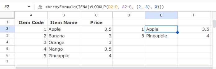
The formula returns a two-column output. We used IFNA to remove #N/A errors at the bottom of the result.
The formula outputs values in E2:F. However, E4:F will have blank cells, preventing you from entering any value in E4:F without breaking the formula.
You can use the LET formula by replacing the placeholder text as follows:
=LET(formula, ArrayFormula(IFNA(VLOOKUP(D2:D, A2:C, {2, 3}, 0))), lastr, ArrayFormula(XMATCH(TRUE, CHOOSECOLS(formula, 1)<>"", 0, -1)), FILTER(formula, SEQUENCE(ROWS(formula))<=lastr))Why Not Use FILTER or TOCOL for This?
Some of you may have seen the use of the FILTER function to filter out blank rows in the formula results. However, keep in mind that it will filter out blank rows throughout the result, not just from the bottom.
The TOCOL function can also remove blank cells, but it is specific to a single column.
Therefore, you can use my all-weather formula to filter out extra blank cells at the bottom of single or multiple-column ARRAYFORMULA results in Google Sheets.
Resources
Here are some Google Sheets resources that discuss the topic of blank rows.
- How to Count Until a Blank Row in Google Sheets
- How to Get Rows Excluding Rows with Any Blank Cells in Google Sheets
- Count From the First Non-Blank Cell to the Last Non-Blank Cell in a Row
- How to Sort Rows to Bring the Blank Cells on Top in Google Sheets
- Filter Out If the Entire Row Is Blank in Google Sheets


