To write cumulative sum, aka running total array formula in Google Sheets, we can use functions such as SUMIF, DSUM, MMULT, and SCAN (LHF). In this tutorial, I’ve included formulas based on all of them.

I’ve extensively used such calculations to plot S Curves as part of generating daily Progress Reports (DPR) related to my job.

Here I am providing you with six different formulas to do cumulative sum (CUSUM) in Google Sheets.

In this tutorial, you will get two non-array and four array-based running total formulas to use in Google Sheets.

In real life, there are several instances where we can use a cumulative sum. We can consider a Cricket match score as an example.

In a Cricket match, the total score is the summation of the Runs.

Each time a player scores runs, it is added to the total.

Column C in the below screenshot is an example of a CUSUM in a Cricket match.

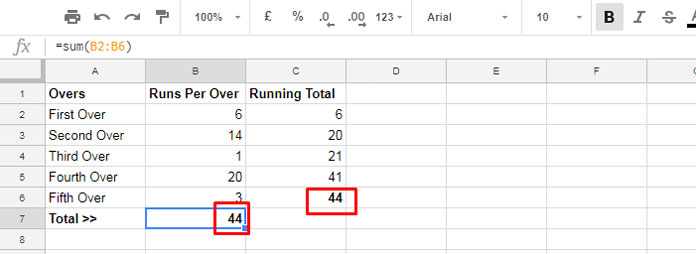
If you are not familiar with the Cricket game, you can ignore everything except the numbers in the above sample data.

You only need to understand that the sum of B2:B6 (B7) is equal to the value in C6, which is derived from the summation of a sequence of runs/numbers in B2:B6.

Here column C contains the running total of the numbers in column B.

Normal Running Total (Cumulative Sum) Formulas in Google Sheets

1. Using the Addition Operator

Here is the basic or the simplest form of running the total calculation in Google Sheets.

Steps:

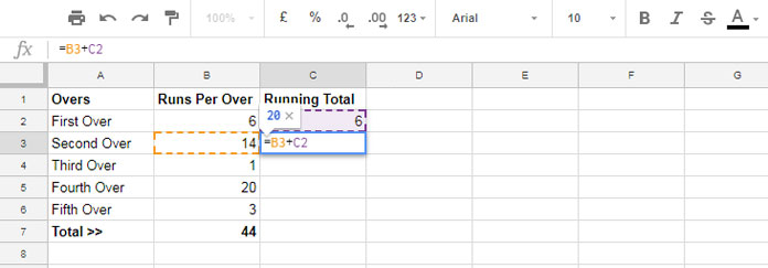
1. In cell C2 insert =B2.
2. In cell C3, insert the formula shown in the image, i.e., =B3+C2, and drag it down.

Your CUSUM is ready.

2. Using the SUM Function

Here is another similar approach to getting the CUSUM in Google Sheets.

This is a tricky use of the SUM function.

You can use the below formula directly in cell C2 and then drag it to the rows down.

=sum($B$2:B2)

Here, the use of the dollar symbol makes the first part of the referenced cell absolute. The second part is relative.

After copying this formula down, check the formula in cell C3. It would be as follows.

=sum($B$2:B3)

I hope it makes sense.

Now let us see how to code running total array formulas in Google Sheets.

Array-Based Running Total Formulas in Google Sheets

As I have mentioned, we can use different functions here, such as SUMIF, MMULT, DSUM, and SCAN.

Among the four, SUMIF is the popular choice of many Google Sheets users and SCAN is the latest in the foray.

1. Cumulative Sum Array Formula Using SUMIF

A one-line array formula can return CUSUM in Google Sheets.

You only need to key the below formula in cell C2 (empty C2:C first).

=ArrayFormula(If(len(B2:B),(SUMIF(ROW(B2:B),"<="&ROW(B2:B),B2:B)),))

Formula Explanation:

The core part of the above CUSUM formula is the SUMIF function.

Syntax: SUMIF(range, criterion, [sum_range])

First, let’s see the role of the ROW function, which acts as the range and criterion within the SUMIF here.

In the following example, the range is E2:E6, the criterion is “<=”&F2:F6, and the sum_rage is G2:G6.

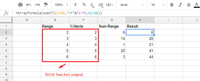
The running total array formula in cell H2 uses these values and returns the cumulative sum.

Logic:

For example, in cell E4 (range), the value is 4. The formula checks whether this value is <= the value in F2:F6 (criterion).

It evaluates to TRUE in the range/array F2:F4, so the SUMIF totals column G up to that range and returns 21 in H4.

2. Cumulative Sum Array Formula Using MMULT

We can use MMULT for writing a cumulative sum array formula in Google Sheets.

As per the above example, we can use the following MMULT formula for returning CUSUM in Google Sheets.

=ArrayFormula(MMULT(IF(ROW(B2:B6)>=TRANSPOSE(ROW(B2:B6))=TRUE,1,0),B2:B6))

For the formula explanation, please check my guide – Running Total Array Formula in Excel [Formula Options].

Here in Google Sheets, I have additionally used the ArrayFormula function together with MMULT.

But when using its competitor application, you may enter the formula using Ctrl+Shift+Enter (legacy array method), or if you are using Office 365, it may spill the result by default.

In Google Sheets, we can use an open range starting from any row in formulas.

So, you may want to make B2:B6 open.

In that case, you can use the below MMULT-based running total array formula in Google Sheets.

=ArrayFormula(if(len(B2:B),MMULT(IF(ROW(B2:B)>=TRANSPOSE(ROW(B2:B))=TRUE,1,0),n(B2:B)),))

It might be resource hungry. So I don’t recommend using it.

3. Running Total Array Formula Using DSUM

The DSUM function is another option to code a running total array formula in Google Sheets. It’s a database function.

So we should format the numbers in the range B2:B6 to 1-12-123-1234 pattern within DSUM. It turns out to be the database for calculation.

We have followed similar approaches earlier using functions such as DMIN and DMAX (please refer to “Related Topics” 9 and 10 below).

I am copying the same formula used there. The only difference is the function in use and cell range (array) reference.

=ArrayFormula(DSUM(transpose({B2:B6,if(sequence(5,5)^0+sequence(1,5,row(B2)-1)<=row(B2:B6),transpose(B2:B6))}),sequence(rows(B2:B6),1),{if(,,);if(,,)}))

Here also you can make the cell range B2:B6 open. You can find the details within those two tutorials.

4. Running Total Array Formula Using SCAN (LHF)

SCAN is a new entrant into the foray of cumulative sum array formulas in Google Sheets.

It’s a LAMBDA helper function (LHF), the simplest way to code an array formula to return the running total in Google Sheets.

For a closed range, the below code will do the magic!

=scan(0,B2:B6,lambda(a,v,(a+v)))

When you want to open B2:B6 to B2:B, use it as follows.

=ArrayFormula(if(B2:B="",,scan(0,B2:B,lambda(a,v,(a+v)))))

That’s all about CUSUM formulas in Google Sheets. Thanks for the stay. Enjoy!

Sample_Sheet_CUSUM

Thanks for the stay. Enjoy!

Related Topics:-

1. Array Formula for Conditional Running Total in Google Sheets.
2. Reverse Running Total in Google Sheets (Array Formula).
3. How to Calculate Running Balance in Google Sheets.
4. Cumulative Balance against Each Payment in Google Sheets.
5. Running Count of Multiple Values in a List in Google Sheets.
6. Running Count in Google Sheets – Formula Examples.
7. Cumulative Count of Distinct Values in Google Sheets (How-To).
8. Reverse Running Count Simplified in Google Sheets.
9. Running Max Values in Google Sheets (Array Formula Included).
10. Find the Running Minimum Value in Google Sheets.