Whether you have a login and logout date-time or time in and time out date-time in a column in two separate rows, you can consolidate them into the same row.
We will use a combination formula mainly based on FILTER and REDUCE to combine time in and time out into the same row in Google Sheets.
Features:
- The formula can combine time in and out for multiple persons/IDs.
- It can handle multiple time-ins and time-outs by the same person/ID.
- No issue if only time in is recorded, and time out is pending.
- The formula returns the entire result as a table.
Drawback:
The formula has one drawback. If you have a very large data set, the formula may fail as it utilizes one of the lambda helper functions, REDUCE.
In that case, you may consider splitting your source data into multiple tables and using multiple formulas.
You May Like:- How to Create Self-Formatting Tables in Google Sheets (With a Simple Initial Setup)
Sample Data and Requirements
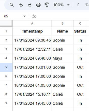
For our sample data, we need three columns: a timestamp column, an ID column, such as employee ID or Name, and a status column containing the strings “In” or “Out.”
In our sample data, column A contains timestamps (in and out times), column B contains the names of a few employees, and in column C, you can find the recorded time as either “In” or “Out” (status).
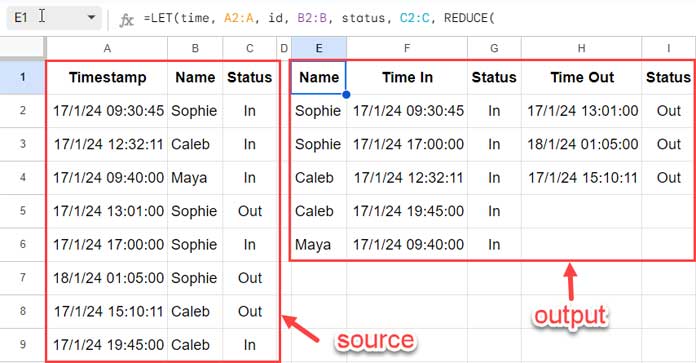
We will implement an array formula in cell E1 that consolidates the time in and out for all individuals in this sample data into their respective rows.
The formula will return the persons’ names in one column and their time in and time out in two separate columns. Please refer to the image below for the combined in and out results.
How to Combine Time In and Time Out into the Same Row in Google Sheets
Here is the ‘hidden’ formula in cell E1 that returns the results in columns E to I in the order of “Name,” “Time In,” “Status,” “Time Out,” and “Status.”
=LET(time, A2:A, id, B2:B, status, C2:C, REDUCE(
     HSTACK("Name", "Time In", "Status", "Time Out", "Status"),
     TOCOL(UNIQUE(id), 3),
     LAMBDA(accu, row,
          IFERROR(VSTACK(
               accu,
               HSTACK(
                    SORT(FILTER(HSTACK(id, time, status), id=row, status="In")),
                    SORT(FILTER(HSTACK(time, status), id=row, status="Out"))
               )
          ))
     )
))
This formula tends to convert timestamps to date values due to the use of the IFERROR function. Therefore, when applying this formula, select the login/logout or time in/time out columns in the result range and apply Format > Number > Date time.
In the formula explanation section below, I have provided details on how this formula combines the time in and time out into the same row in Google Sheets.
The Logic Behind the Formula that Combines Time In and Time Out in Google Sheets
The logic of the formula that combines time in and time out into the same row is very simple. What makes it complex is the application of the logic using the REDUCE Lambda function.
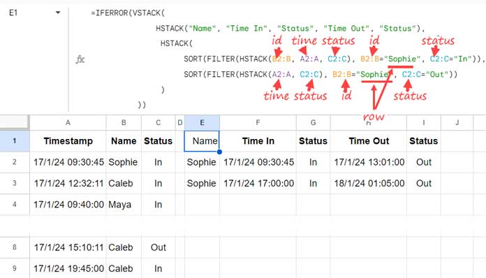
There are two filters in the formula:
The first filter selects the rows matching a particular person with the status “In” and sorts them, placing the earliest records at the top.
The second filter selects the rows matching the same person with the status “Out” and sorts them, placing the earliest records at the top.
Stack these results horizontally. The outcome will be the combined in and out times for a particular person. We use REDUCE to efficiently apply the logic to the time in and out for all persons.
Breaking Down the Formula:
We have utilized the LET function to assign meaningful names to each column in the data. Here is the syntax of the LET function and the ranges with their assigned names.
Syntax:
LET(name1, value_expression1, [name2, …], [value_expression2, …], formula_expression)Names and Value Expressions:
time, A2:A,
id, B2:B,
status, C2:C
We will use the names (time, id, and status) instead of the ranges (A2:A, B2:B, and C2:C) in the REDUCE.
Formula Expression:
REDUCE(
     HSTACK("Name", "Time In", "Status", "Time Out", "Status"),
     TOCOL(UNIQUE(id), 3),
     LAMBDA(accu, row,
          IFERROR(VSTACK(
               accu,
               HSTACK(
                    SORT(FILTER(HSTACK(id, time, status), id=row, status="In")),
                    SORT(FILTER(HSTACK(time, status), id=row, status="Out"))
               )
          ))
     )
)
To understand the formula expression, which is essentially a REDUCE formula, let’s first review its syntax.
REDUCE Syntax:
REDUCE(initial_value, array_or_range, lambda)Now, let’s break down how the REDUCE formula combines time in and time out into the same row in Google Sheets.
initial_value:HSTACK("Name", "Time In", "Status", "Time Out", "Status")represents the title we want to return at the top of the result.array_or_range:TOCOL(UNIQUE(id), 3)represents unique names.LAMBDA(accu, row, …): Defines a lambda function taking two parameters (‘accu’ and ‘row’). The initial value in the ‘accu’ (accumulator) is the title for the result, and the ‘row’ represents each element in the array (unique names).
Here is what the function does:
IFERROR(VSTACK(
               accu,
               HSTACK(
                    SORT(FILTER(HSTACK(id, time, status), id=row, status="In")),
                    SORT(FILTER(HSTACK(time, status), id=row, status="Out"))
               )
          ))
It vertically stacks the accumulator value (initially the title row) with horizontally stacked two sorted filtered results.
- The first FILTER filters the data where ‘id’ (B2:B) equals the current ‘row’ value in
TOCOL(UNIQUE(id), 3), and ‘status’ is “In.” - The second FILTER filters the data where ‘id’ (B2:B) equals the current ‘row’ value in
TOCOL(UNIQUE(id), 3), and ‘status’ is “Out.”
The REDUCE function iterates through each element (represented by ‘row’) in the array (TOCOL(UNIQUE(id), 3)), ensuring that the FILTERs filter all the unique names.
Resources
This tutorial elaborated on combining time in and time out into the same row. Here are some related tutorials that address joining two tables. They also utilize the REDUCE and FILTER combo but in a different fashion.


Hi All,
I’ve revised the formula used earlier as we now have better options with Lambda. Please go through the tutorial.
What if the time out is the next day?
Example:
Time In: 02/15/2023 17:00:00
Time Out: 02/16/2023 00:30:53
The formula only works for the same day.
Hi, Ivan,
You can use the below formula. It won’t work if a person has two or more logins and logouts.
=map(A2:A9,lambda(_,if(countif(A2:_,_)=1,xlookup(_,A2:A9,B2:B9,"",0,-1),)))Very Good. But what about if there is No “IN” or “OUT”?
How to move the second entry in a day of the same employee as the OUT time?
I am desperately searching for that.
Hi, Prakash,
Assume you don’t have the “Status” column C.
If so, empty C1:C and insert the below running count in C1.
=ArrayFormula({"Running Count";if(A2:A="",,countifs(row(A2:A),"<="&row(A2:A),A2:A&int(B2:B),A2:A&int(B2:B))) })
Empty F1:H for the output.
Formulas:
F2
=filter(A2:B,C2:C=1)
H2
=ArrayFormula(ifna(vlookup(F2:F&int(G2:G),{filter(A2:A,C2:C=2)&int(filter(B2:B,C2:C=2)),filter(B2:B,C2:C=2)}
,2,0)))
If the above doesn't help, you can make a sample and share its URL below.