


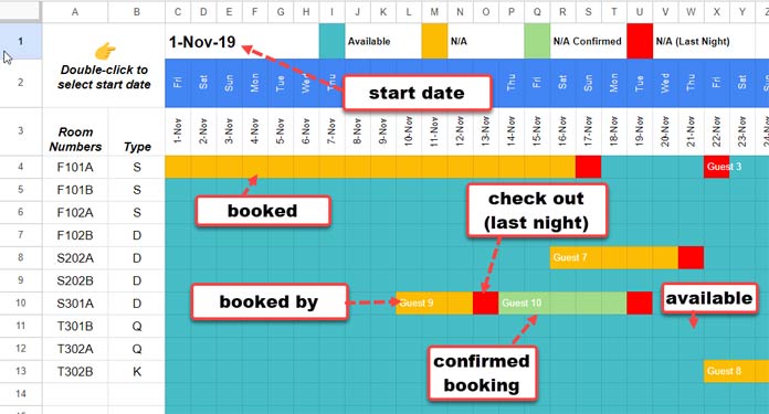
My reservation and booking status calendar template in Google Sheets uses spreadsheet cells as rooms and highlighting to show availability/non-availability.
I have used a few formulas and conditional formatting rules. All the formulas are array formulas, so you do not need to worry about copying and pasting when you add more data.
How-to guides are the highlights of this blog. So in this post, in addition to providing a link to my reservation and booking calendar template, I have also included the how-to part of it.
These have two benefits:
- If you are not familiar with complex Google Sheets formulas, you can use the template as is. I have provided the instructions within the template and in this post.
- If you have some idea about Google Sheets formulas, you can follow my how-to part to customize the template for your own different purposes.
My template is meant for monitoring hotel reservation/booking status, such as the availability and non-availability of rooms. However, you can use the template if you want to book anything similar, such as viewing the status of program/event booking or the status of rent-a-car booking.
First, get my Google Sheets reservation/booking status calendar template so that I can explain how to use it.
Reservation and Booking Calendar Template in Google Sheets: Features
First and foremost, this template is free and easy to use, even with limited Google Sheets (spreadsheet) knowledge. It also allows you to easily find the availability of rooms on any particular date or date range.
Here are the key features:
- The template can show three months of booking data based on a provided start date. You can choose different start dates.
- I have added rows for 50 rooms, but you can add more rows if you have more rooms.
- I used conditional formatting to show the availability (light blue) or unavailability (orange, light green, or red) of rooms. Since this is basically a hotel room reservation and booking calendar template, it uses booked nights. So if a person booked a room from November 16, 2019 to November 22, 2019, the highlighting will be as follows:
- November 16, 2019 to November 20, 2019: 5 days in orange if the booking is tentative and light green if the booking is confirmed.
- November 21, 2019: 1 day in red. No highlighting will be on the 22nd as that day is available for the next booking. (You can modify these three rules to highlight the start date to the end date if your purpose is something different.)
- The booking person’s name (guest) is shown in the chart.
The above are the key features of my reservation and booking calendar template in Google Sheets.
This makes it easy to find the availability of rooms on any particular date or date range.
How to Use the Reservation and Booking Status Template in Google Sheets for Your Business
The reservation and booking status calendar template in Google Sheets uses two Sheets within a file:
- Availability
- Reservations
There is also a third tab named “Notes,” which is self-explanatory. Let me explain what you may need to change/adjust in each sheet:
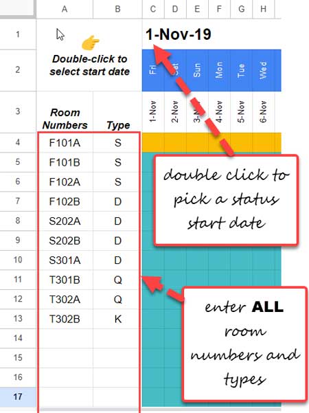
1. Availability Sheet: How to Customize It to Meet Your Needs
The “Availability” sheet is the homepage of the booking and status calendar template. In this sheet, you can see the statuses of bookings and availability in the range C4:CP53.
There is some dummy data in A4:B53. Replace them with your own data: room numbers (A4:A53) and room types (B4:B53), but room types are optional.
You can add up to 50 room numbers because the range in A4:A53 is 50 rows. If you have more rooms, simply add more rows at the bottom.
You only need to make one more change. There is a date picker in cell C1. This controls the date range for the chart C3:CP3.
2. Reservations Sheet: How to Customize It to Meet Your Needs
The “Reservations” sheet is for entering your booking data. You can keep all your booking data (previous, current, and upcoming) on this sheet.
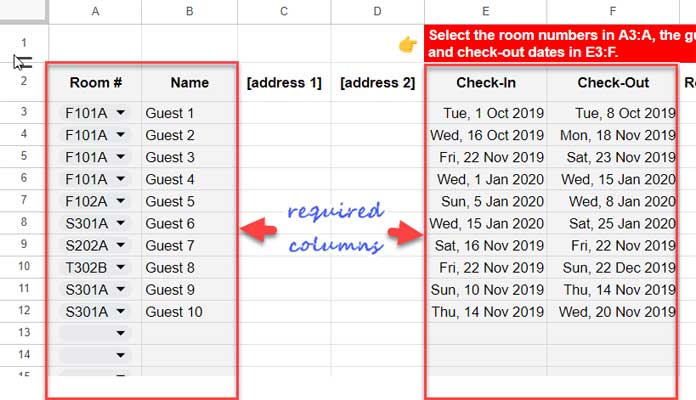
You are required to enter or select the following data:
- Pick room numbers in A3:A (The drop-downs will be populated with all your room numbers in
Availability!A4:A53). - Enter the check-in date in E3:E and the check-out date in F3:F.
- Enter the booking name in B3:B.
- In cells H3:H, select the booking status from the two options: Confirmed and Tentative. Their bar colors will be light green and orange, respectively. However, if the booking is for one night, these rules will be overridden and the color will be red.
Please take extra care when entering data in this sheet. Avoid duplicate entries. For example, if a room is booked from January 1, 2023 to January 31, 2023, the same room should not be booked for any date in that date range.
This is important because the purpose of the reservation and booking calendar template is to check the availability of rooms.
To avoid duplicate entries, check the Availability sheet chart area for the room’s availability before entering each booking. You should also pick the appropriate date in Availability!C1.
Note: You can insert or delete columns only after column H.
How to Create a Booking Calendar Template in Google Sheets
In this section, I will share the formulas used in both the “Availability” and “Reservations” sheets and their purposes. I hope this will help you modify the formulas if needed.
1. Formula in the Reservations Sheet
In cell G2 of the “Reservations” sheet, I have the following array formula, which populates the number of days booked from the check-in and check-out dates of guests:
=ARRAYFORMULA(VSTACK("Room Nights",IF(A3:A="",,DAYS(F3:F,E3:E))))Note: We don’t need this formula to create the bars in the “Availability” tab of the reservation and booking calendar.
Formula Explanation:
- The DAYS function is used in an array formula to calculate the number of days between the check-in and check-out dates for each room.
- The VSTACK function creates a vertical stack of two arrays: the first array contains the header text “Room Nights” and the second array contains the number of room nights returned by the DAYS function.
- The IF function checks if the room number in column A is empty. If it is empty, the function returns a blank value. Otherwise, the function returns the number of days between the check-in date (column E) and the check-out date (column F) for that room.
2. Formulas in the Availability Sheet
We have used the following SEQUENCE formula in cell C3 to populate the third row in C3:CP3 with three months of dates (timescale):
=SEQUENCE(1,DAYS(EDATE(C1,3),C1),C1)How does this formula work?
The EDATE(C1,3) function in the formula returns a date that is three months after the start date in cell C1.
The SEQUENCE function returns sequence numbers in one row and n columns, starting from the date in cell C1. The value of n is determined by the number of days between the date in C1 and EDATE(C1,3).
The following C2 formula converts the populated dates in C3:CP3 to the days of the week:
=ARRAYFORMULA(IF(LEN(C3:3),TEXT(C3:3,"ddd"),))The following C4 formula in the “Availability” sheet fetches the booking names from the “Reservations” sheet and places them in the check-in date cells:
=LET(
   dt,C3:3,
   room,A4:A,
   guest,Reservations!$B$3:$B,
   r_room,Reservations!$A$3:$A,
   start,Reservations!$E$3:$E,
   MAP(dt,LAMBDA(c, MAP(room,LAMBDA(r,
      JOIN(" ?",IFNA(FILTER(guest,(r_room=r)*(start=c))))
   ))))
)
Formula Explanation:
The LET function defines five variables:
dt: The dates in row 3 of the “Availability” sheet.room: The room numbers in column A of the “Availability” sheet.guest: The guest names in column B of the “Reservations” sheet.r_room: The room numbers in column A of the “Reservations” sheet.start: The check-in dates in column E of the “Reservations” sheet.
The MAP function is used to iterate over the dates in dt and the room numbers in room, both in the “Availability” sheet.
For each date (dt) and room number (room), the MAP function uses the FILTER function to filter the guest names in guest (“Reservations”) to only include the names of guests who have booked that room on that date. The result of the MAP function is a two-dimensional array.
The JOIN function joins the filtered guest names into a string, separated by commas (it is part of troubleshooting because there won’t be two names on the same booking date for the same room).
3. Conditional Format (Highlighting) Rules in the Availability Sheet
Highlight rules are essential in creating a visually appealing reservation and booking calendar template in Google Sheets.
We have three conditional formatting rules for the range C4:CP53. To see them, click on cell C4 and go to Format menu > Conditional formatting.
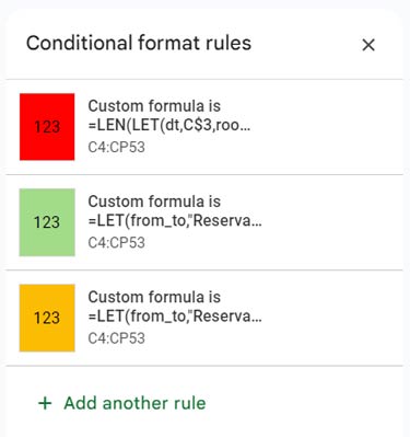
The first rule fills the cells corresponding to the booked dates in the timescale (C3:CP3) with an orange color for tentative bookings based on column H in the Reservations sheet.
The second rule replaces the orange color with a light green color for confirmed bookings, also based on column H of the Reservations sheet.
The third rule highlights the night before checkout with a red color (not the checkout date itself). So, if the booking is for one night, the color will be red, not light green or orange.
Here are those formulas (rules used for the range C4:CP53):
Booked Days (Orange)
=LET(
   from_to,"Reservations!E3:F",
   booked_room,"Reservations!A3:A",
   status,"Reservations!H3:H",
   room,$A4,
   dt,C$3,
   ftr,FILTER(INDIRECT(from_to),(INDIRECT(booked_room)=room)*
   (INDIRECT(status)="Tentative")),
   SUM(
      MAP(CHOOSECOLS(ftr,1),INDEX(CHOOSECOLS(ftr,2)-1,0),
      LAMBDA(st,en, N(ISBETWEEN(dt,st,en))))
   )
)
This Google Sheets formula is the essence of the reservation and hotel room booking template. It draws the bar for the booked days in the chart area. How?
Formula explanation:
The LET function defines four variables:
from_to: The range of cells in the “Reservations” sheet that contain the check-in and check-out dates for each booking.booked_room: The range of cells in the “Reservations” sheet that contain the room numbers for each booking.status: The range of cells in the “Reservations” sheet that contain the statuses of each booking.room: The room number in A4 of the “Availability” sheet.dt: The date in C3 of the “Availability” sheet.
The FILTER function filters the from_to range to only include the rows where the room number in the booked_room range matches the value of the room variable and the status of the booking is “Tentative”.
The CHOOSECOLS function separates the filtered from_to range into two parts: start and end dates, named st and en within the LAMBDA in MAP.
The MAP function iterates over the st and en within ISBETWEEN to test if the dt (C$3) falls in that range. The output will be TRUE or FALSE, which the N function converts to 1 or 0, respectively. The SUM function returns the total of it.
If the total is greater than 0, that cell is highlighted.
Since it’s a highlights rule and in room ($A4) the column is fixed and in dt (C$3) the row is fixed, it automatically applies to all rooms and dates in the chart.
Booking Confirmation (Replaces Orange with Light Green)
The same “Orange” rule was copied and modified with the following changes:
The FILTER function was updated to replace the condition “Tentative” with “Confirmed”.
Filter condition in Orange Color Highlighting:
(INDIRECT(status)="Tentative")Filter condition in Light Green Color Highlighting:
(INDIRECT(status)="Confirmed")Last Night (Red)
=LEN(LET(
    dt,C$3,
    room,$A4,
    guest,"Reservations!$B$3:$B",
    r_room,"Reservations!$A$3:$A",
    end,"Reservations!$F$3:$F",
    IFNA(FILTER(INDIRECT(guest),(INDIRECT(r_room)=room)*
   (INDIRECT(end)-1=dt)))
))
Formula explanation:
The LET function defines five variables:
dt: The date in C3 of the “Availability” sheet.room: The room number in A4 of the “Availability” sheet.guest: The range of cells in the “Reservations” sheet that contain the guest names for each booking.r_room: The range of cells in the “Reservations” sheet that contain the room numbers for each booking.end: The range of cells in the “Reservations” sheet that contain the check-out dates for each booking.
The FILTER function filters the guest range to only include the rows where the room number in the r_room range matches the value of the room variable and the check-out date in the end range -1 is equal to the given date (dt).
The IFNA function is used to handle the case where there are no guests who have booked the room on the given date. In this case, the IFNA function returns an empty string.
The LEN function returns the length of the string returned by the IFNA function. If the output is greater than 0, the formula highlights the cell.
This rule is applied to the whole chart area. Since the dt (C$3) variable uses an absolute row and the room variable uses an absolute column, it applies to all the ranges in the chart area.
Booking Calendar Template: How to Consider the Check-Out Date (Not Last Night)
Some users may want to highlight the booking start date to the end date (from the check-in date to the check-out date). Above, we considered booked nights.
To make this change, you only need to remove the -1 from the orange, light green, and red highlight rules. You can scroll up to see the formulas where I have highlighted them.
I hope you like this free reservation and booking calendar template! Here are some other popular templates:
Hi, how I can make so that the name of the guest is repeated in every single cell of the green stripe?
To ensure the guest’s name is repeated in every cell of the green/red (booking confirmed) stripe, I recommend replacing the formula in C4 with the following:
=ArrayFormula(LET(dt,C3:3,
room,A4:A,
guest,Reservations!$B$3:$B,
r_room,Reservations!$A$3:$A,
start,Reservations!$E$3:$E,
end,Reservations!$F$3:$F,
status,Reservations!$H$3:$H,
MAP(dt,LAMBDA(c, MAP(room,LAMBDA(r,
JOIN(" ?",IFNA(FILTER(guest,(r_room=r)*(status="Confirmed")*(GTE(c,start))*(LT(c,end)))))
))))
))
If you also want the name in the orange/red (tentative) stripe, remove the
(status="Confirmed")*part from the formula.Thank you!
Hello, I encountered an issue and I was hoping you could help me. A client has reserved more than 10 days, and the start day until the end day in the availability sheet cannot be seen on one page, causing the blue bar to be out of view. How can we position the blue bar so that it’s visible?
Feel free to share a copy via email or share the URL below. That will help me understand the real scenario.
Hello,
Thank you for the sheets and the effort you put into them.
I would like to ask for advice. I’m interested in counting the number of people in the hotel for each date, and if possible, separating those who have confirmed from those who are “tentative”.
Is there a way to accomplish this?
Thank you.
In a new sheet, enter the following formula in cell A1:
=ArrayFormula(QUERY(SPLIT(FLATTEN(Reservations!H3:H&"|"&MAP(Reservations!E3:E, Reservations!F3:F,
LAMBDA(x, y, SEQUENCE(1, y-x+1, x)))),"|"),"SELECT Col2,
COUNT(Col2) WHERE Col2 IS NOT NULL GROUP BY Col2 PIVOT Col1", 0)
)
Please note that this is a resource-intensive formula that will possibly return a three-column output. The first column will consist of date values. Select the first column and apply Format > Number > Date.
The formula calculates the number of nights booked for each date, with confirmed and tentative bookings displayed in separate columns.
Thank you for your quick reply,
I would prefer something that can be shown directly on the Availability screen. In my situation, I want to include three lines above the room number and booking calendar (lines 4, 5, and 6). Line 4 should display the total, line 5 should display the number of confirmed bookings, and line 6 should display the number of tentative bookings. I want every line to be filled, even when the number is 0.
Sorry, I don’t know how to send an image of what I want, but I hope I explained it correctly.
You can potentially utilize my above formula as the source and lookup values from it using XLOOKUP in the Availability Sheet. However, I am not in favor of using complex formulas since the sheet is already heavily loaded with functions and highlighting rules.
Thank you very much
Hi Prashanth,
Thank you for providing the calendar template. Is it possible to modify the check-in/check-out date format to mm/dd/yy? I attempted to change the format, but it resulted in an error.
Additionally, could we explore the option of adding more statuses (Confirmed/Tentative)? I’m interested in incorporating statuses for Male, Female, and Private Room.
You can adjust the date format by following these steps:
Click on File > Settings and change the Locale to United States. Save the Settings.
Next, select cells E3:F in the “Reservations” sheet and click Format > Number > Date.
Please note that adding extra statuses is not recommended, as it necessitates additional highlight rules and could potentially impact performance.
Any suggestions on how to edit it to manage bookings with hourly slots?
Sure, I’ll work on a template for managing bookings with hourly slots. I’ll post it as soon as possible. Please stay tuned!
Please check out this Hourly Time Slot Booking Template in Google Sheets.
The calendar template you provided is wonderful, but I’m aiming for a more detailed view. While the three-month calendar layout is helpful, I was wondering if there’s a version that offers a weekly overview with a more detailed breakdown of days by hours. Having the ability to view and manage bookings on a daily basis with hourly slots would be incredibly beneficial.
I apologize. Currently, such a template is not available. I will consider this for future development.
Hi everyone,
I’ve updated the reservation and booking status calendar template, adding new features and removing the helper tabs to make it more user-friendly.
Please check it out and let me know what you think!
Hi Prashanth,
I am writing to you today to inquire about a feature that would allow me to detect room overlaps in the Tab Availability sheet.
For example, if I have a room that is booked for the dates of 06/07/2023 – 10/07/2023 and then I book the same room for the dates of 08/07/2023 – 12/07/2023, the Tab Availability sheet would not currently show this as an overlap.
I would like to know if there is a way to modify the color of the cell if there is an overlap in room bookings. This would help me to easily identify any potential conflicts.
Thank you for your time and consideration.
Hi Dewa,
I understand your concern. I don’t want to add any more formulas to the sheet because I’m concerned that adding more formulas could affect the performance of the sheet.
Thank you for your understanding.
Hi,
Thanks for this! Really helpful.
By the way, how to expand this to cover say, 4 time block for each day?
As I’m trying to figure out a schedule for a car rental
Hi, mjj4884,
This template is not suitable for that.
Thanks.
Hi, Prashanth!
My table breaks when entering more than 20 rows of data. Why can this be? Instead of filled-in cells, I get numbers in them, and formulas are not fully loaded.
Hi, Nar,
Thanks for sharing your example Sheet. But it doesn’t reflect the problem.
Also, I suggest you remove the rule for highlighting in “Filtered” for improved performance.
After I try to add data to the table, there is an infinite loading.
Hi, Nar,
That might be due to the conditional formatting mentioned earlier. I’ve removed that. Please try again.
Hi, Prashanth!
Thank you for your work!
Hi Prashanth. Thank you for that, but there is still a glitch in one of the rooms in row 5 where it appears to be continuously booked ( all boxes are orange/yellow) even though it isn’t.
Waiting for your response within the Sheet.
Resolved. Thanks for your support.
Thank you for your time and effort Prashanth
– URL removed by the Admin –
The dates in the “availability” and I and J columns in “reservations” do not correspond to the dates I filled in.
I have also sent you emails.
Hi, Nick,
Please share the URL with Editable rights. Also, I haven’t received your email.
Thanks. I got the file and updated the formulas to cover six months of data.
Hi Prashanth,
The file won’t take any dates of reservations after line 21.
The dates I put in the reservation section/spreadsheet do not come in the availability section/spreadsheet.
Hi, Nick,
Can you share that file?
Share mockup data only.
Hi Prashanth,
Did you get the file?
I didn’t. You can share it (URL) below. I won’t publish that comment.
Hi Prashanth,
Thank you so much for this very handy tool. I would like to record my bookings for more than 3 months in advance, can you please advise how I could achieve this.
Will I need a different spreadsheet for each 3-month period, or is there a way to extend the duration?
Hi, Nick,
You can record your bookings for more than 3 months. The VIEW is only limited to three months.
I suggest you view the booking part by part. For example, enter 1-1-2023 in cell Availability!C1 to view the bookings from 1st Jan to 31st March.
Then enter 1-4-2023 in that cell to view the next three months’ bookings.
Thanks for the reply. My 3-month period is currently set at 17/3/2023 to 16/6/2023.
I tried changing the start date to 17/6/2023, but all my bookings from March were moved forward and appeared in June.
It seems I have messed something up.
Can I share the file with you so can take a look at it?
Please advise
Hi, Nick,
OK, if you want to visualize six months of data in one go, do as follows.
Note:- I don’t advise it as it can impact your Sheets’ performance.
1. Enter
=sequence(1,200)formula in Filtered!D2.2. Enter
=edate(C1,6)-1formula in Availability!G1.3. Replace
Filtered!$D$3:$CYpart of the Availability!C4 formula withFiltered!$D$3:$GU.Please try it and let me know.
Is there a way to keep the check-in and out-date cells blank (E1:F) in the reservations while maintaining the drop-down function and your custom formula?
I don’t want all dates showing until I input a value. I’ve tried adding a rule, but I keep breaking something.
Hi, Luca,
Sorry! I’m not clear 🙁
Great, I understand.
“You can use Data (menu) > Data Validation to avoid accidentally entering values.”
How do I do this exactly?
Hi, Ariel,
1. Click on cell D4
2. Go to the Data menu Data validation
3. Select “Add rule”
4. Apply to Range (as per my template range):
Availability!D4:CP13,Availability!C5:C135. Criteria: “Custom formula is”
And here is the formula to use there.
=not(len(D4))It may leave error symbols in highlighted cells. Just ignore it.
I hit delete in V5, and it worked! Thank you!
The thing is that I do not understand your first sentence, where I think you describe what the problem was.
What was wrong? How can I avoid this happening again in the future?
Thank you very much for your help!
Hi, Ariel,
You can find an array formula (expanding formula) in cell C4.
The value in cell V5, which you may have accidentally entered, prevented it from working.
Do not enter values in cells other than the specified area. You can use Data (menu) > Data Validation to avoid accidentally entering values.
Hi Prashanth,
Here it is:
* URL Removed By Admin *
I put dummy names and left a few records so you can analyze them.
Thank you very much, Prashanth. I look forward to seeing what the problem is and solving it!
Keep up your great work,
Ariel.-
Hi, Ariel,
All the cells except C4 in the range Availability!C4:CN9 must be blank.
Go to Availability!V5 and hit the Delete button. That may solve the issue.
Hello Prashanth,
Thank you for your reply!
I read your reply to Kerim, but I do not see a solution to my problem.
I can see the red highlight (last day of occupancy) but not the highlight for the other days. I think Karim is having another problem.
Would it be possible to send you the link so you can take a look?
Thank you very much!!
I look forward to using this great tool once it´s working again.
Best regards,
Ariel.
Hi, Ariel,
Please send it but only with a few records for fast-loading the file.
Also, replace real names with dummy names.
Hello Prashanth,
First of all, thank you for your work.
I have a problem with the availability sheet because it shows the reserved days and then not anymore (just the red one showing the last night).
Could you please help me? THANK YOU!!
Hi, Ariel,
Please go through my reply to Kerim.
Amazing template Prashant, thank you.
I successfully multiplied everything except the last night highlighting in red color. I can’t seem to find where the problem is. This is the only problem that holds me from using it. Could you please have a look?
— URL removed by Admin —
Hi, Kerim,
The issue is the special characters in room numbers.
Also, to improve the performance of the Sheet, you can remove the highlighting in the “Filtered” tab.
Hell,
Thank you for this template. I have a suggestion for improvement.
Sometimes we have rooms in the hotel for monthly rent, and I need a table that shows me the availability of rooms on a monthly schedule in the same way the daily schedule was shown.
Hey Prashanth,
A very nice template you’ve made.
However, I found an issue when there is a reservation on the last day that is displayed on the availability sheet.
Example:- When the displayed date is 1-Dec-2022 to 28-Feb-2023, and there is a reservation on the 28th Feb 2023, the whole row on the availability sheet will show the number 0.
Any idea on how to solve this?
Thank you.
Hi, Abu,
The answer lies in row#5 in the “Reservations” tab. Please check G5 there.
The start and end dates must be two different dates to get at least one night’s stay.
Hey Prashanth,
First of all, you are doing great.
I have been using your sheet for the last two months, and it’s been very useful for me.
Many Thanks😃
Hi, Mohamed,
Good to hear that 🙂
What to do when a customer does not give a checkout date? how to display ?
Hi all,
Now there are no drag-down formulas in the template! I’ve updated all of them using the new LAMBDA Helper functions.
Thanks.
Sounds great, Prashanth. What do we need to do to update our existing sheets?
Hi, Anita,
Remove all the formulas in Filtered!D3:D and Availability!C4:C.
Then copy-paste my new array formulas in Filtered!D3 and Availability!C4 from my sample sheet.
Hey Prashanth,
Firstly, great sheet!
We have a small rental shop, and this sheet is just (almost) perfect for us. So thanks!
Is it possible to add the time for check-in and time for check-out, it would help us a lot. A row more is OK, 24-hour time scale.
Also, the Update on April 6, how can we change the formula so the last day (the red color) will actually show on the last day of the booking? Not the night/day before as your formula show. Thanks again!!
Hi Prashanth,
I have been using your template for the last two months, and it’s been so useful.
Now I seem to have an issue. The yellow occupied squares do not show on the Availability tab for some of the rooms.
Could you please have a look and guide me? I’m enclosing the link to my sheet.
— URL of the Sheet removed by admin —
Hi, Anita,
The main issue is the missing formulas in some of the cells in Availability!C4:C.
Once you correct that, the highlighting will re-appear.
Another issue you are having is the duplicate entries in the Reservations tab. For example, refer to rows 49 and 51 (room # 7-1).
You can easily find them from the Filtered tab (red highlighted).
Thank you so much for this spreadsheet! It’s been amazing!
I have, however, run into the issue where a random cell on the “Availability” sheet will turn red. It is not reserved, and it does not have dates for those days. Do you know how I can fix this?
SUPER appreciate any insight into fixing this issue. Thanks again!
Hi, Natasha,
Could you copy that sheet and share its URL with me in your comment/reply below?
— URL removed by Admin —
Here you go! I’ve been trying to troubleshoot the problems more. So you can see it currently in cells AS7 and BL8.
Hi, Natasha,
Thanks for sharing your Sheet.
It’s viewable only. So do as follows to solve the issue caused by using sequence numbers as room numbers.
Go to Availability!C4.
Then go to Format > Conditional formatting.
Click on the Red highlighted conditional format rule.
Edit the formula (replace
$A4&C$3with"^"&$A4&C$3&"$"). You can also copy-paste the formula from my post which is updated now.Thanks for letting me know about the problem.
Hey hey! Thanks for your continued help with this!
I just made a copy of the sheet, and unless I’m looking at it wrong, it looks like there are red cells in the middle of reservations in cells 010 and a random one in X4.
Are these supposed to show up?
Hi, Natasha,
Both are correct.
X4 – (ref.: Reservations!F4) check-in on 22/11/2019 and check out on 23/11/2019. So one-night stay on 22/11/19, and that cell got highlighted in red.
O10 – (ref.: Reservations!F11) check-in on 10/11/2019 and check out on 14/11/2019. So last night’s stay was on 13/11/19, and that cell got highlighted in red.
The real issue was the partial matching of room numbers and that was solved with my previous update.
You do not require to copy my Sheet and start again. Just update the formula in your Sheet as recommended.
Hi Prashanth!
Thanks a lot for that template. It’s working great.
I have a use case a bit different than hotel room reservations.
I rent spots (for vans), and there can be up to 3 reservations per spot on the same day.
So, in the Availability tab, I would like to display a number telling me if there are 1, 2, or 3 reservations on that day.
Do you think I could achieve it with your template? Any advice?
Thanks again!
Hi, Laura P,
Sorry! It won’t work.
Hello!
This is a fantastic template and easy to use for beginners like me.
I wonder why the colors on the “Availability” sheet aren’t suddenly working anymore?
Is there a way to check that the formula is still correct? Thank you!
Hi, Patricia Swenson,
There might be errors on the other tabs. If you want me to check, share a copy of the hotel room booking template after removing personal info if any.
Hello,
This is great. I’m just having trouble with a couple of things.
If I put any reservations on the reservations tab lines 19-22, it creates an error that says, “Function SPLIT parameter 1 value should be non-empty.”
Also, it would be wonderful if the availability calendar turned a different color if you accidentally double-book a room.
Why do Reservation tab columns I and J have different dates than what I input in columns E and F?
Thank you for building this!
Hi, Nikki M Calles,
To solve the Split error, go to the ‘Filtered’ tab and copy-paste the D3 formula down as far as you want.
Regarding accidental double booking, please see the last part of the post for an update.
Thank you!
Hi Prashanth,
Thanks for the reply, I think I did not explain my query clearly… I mean the overlapping of check-in and check-out booking.
What I mean is, for example, our check-in is 2 PM (January 1), and check-out is 12 PM the next day (January 2). Then right away there is another guest check-in on the same day (January 2) at 2 PM… As it is, the day is only highlighted as red regardless if there is a guest booking right away or not…
IF we could add one more color we could easily distinguish if that day is checkout only and no guest right away (RED) or… another color indicating that there is another guest (PURPLE maybe) who has booked the room the same day.
Hi, Myson Mark,
Thanks for your explanation. I could understand it clearly from your last comment itself.
If the check-in is 2 PM (January 1), and check-out is 12 PM the next day (January 2), my template will only highlight January 1st that also in red color to indicate that is the last night of that booking. January 2nd will be blank even if it’s the check-out day.
We are just highlighting (counting) the nights. So, there is no questioning of overlapping.
Please check whether you are using my latest template as I have corrected the sheet recently based on user inputs.
If you go through the comments, you might find similar requests from other users which are finally sorted out using the above method.
Thanks a lot Prashanth 🙂
Hi Prashanth,
Thanks for the template.
Is it possible to add one more color for situations where a room check-in and check-out happen on the same day?
Hi, Myson Mark,
That issue is not arising. For example, one guest has booked room # 301A from 10/11/19 (check-in) to 14/11/19 (check-out).
That means four nights’ stay.
On the ‘Availability’ tab, the cells under the dates 10, 11, 12, and 13 (4 nights) will be highlighted, and 13/11/19 (not 14/11/19) will be highlighted in red to indicate it’s his last night.
The date column 14/11/19 will be blank and available for booking.
Hi Prashanth,
I have added more rooms in Availability and dragged the formula in C3 down. But I am getting the #NUM error “Function SEQUENCE parameter 2 value is 0.”
This error shows in one row. The others are fine.
Hi, Anita,
The said error is carried from the ‘Filtered’ tab column D. But no changes required in this tab or in the ‘Availability’ tab.
The reason for the error probably lies in the “Reservations” tab.
There, in columns E and F, you might have entered the same dates for check-in and check-out in one row.
There must be at least one night’s stay. You can find that by checking column G for 0 (zero) room nights.
Thank you, Prashanth! It works beautifully, and I’ve got the hang of it now.
The new double-check-in red alert is very helpful. I’ve downloaded the template again and transferred all reservations to it. Is it possible for the template to auto-update at my end with all the new features you add when you update it at yours?
Also, I wanted to report that the new template is taking ages to calculate formulas. Is it possible to speed this up? I’ve got about 29 reservations on it so far.
And is it possible to see guest names on the Availability tab, perhaps as a popup when we hover or click on a colored block?
Once again, thanks for all your work on this.
Hi, Anita,
I am glad to hear that you liked the template.
For future updates, please bookmark this post and check the last part of it.
I’ll only update it if any user report issues.
The slow performance of the sheet is probably due to the new rule to highlight duplicates. It’s an optional rule. You can remove that by going to the ‘Filtered’ tab.
Finally, sorry to say, it’s not possible with the current settings to add guest names to the Availability tab. Any further modifications to the template may further deteriorate its performance.
So I accidentally deleted the formula for the room nights column. How do I fix this so it will show me how many nights someone is staying?
Hi, Melissa,
Go to the File menu and click Version history and revert to a previous version.
Will I lose the information I have in the file?
Hi, Melissa,
You can first make a copy of the file (File > Make a copy) and then go to version history.
So your data will be safe in the copy.
Hi, Prashanth.
This job could be for operational simplicity very useful, but there is an important detail that almost prevents its use.
Its purpose is to reserve overnight stays.
The availability calendar must be accurate and truthful because it serves as the main visual reference before a reservation is made.
The availability calendar distinguishes what is free from what is not. Due to the characteristics of the platform, each box can show a unique meaning.
The reservation in the calendar therefore should not occupy even the check-out date but only up to the cell that marks the last night booked.
Because the cell should be free for the new night, and the latter should be highlighted to separate contiguous reservations.
The last night of different colors (like the changes requested by Sandy) should exclusively mark the end – the last night – of a reservation.
The same result of the Reservations! Room Nights field showing the exact number of nights equals the number of cells that will mark the reservation. And not one more as is the case now.
I’ve tried but couldn’t get it.
Could you please explain how this can be achieved?
Thank you in advance.
Hi, Francisco,
Based on your request, I’ve updated the template.
There are two changes.
Updated the Filtered!D3 formula (I had suggested the same to Sandy).
Added a new highlight rule in the “Availability” tab to highlight the last night before the check-out day.
N.B.:- Offered a similar formula rule to Sandy also. But that time, we were trying to implement it on the check-out date, so not practical in use).
Thanks for your suggestions.
Thank you, Prashant!
This is it! I appreciate the modification.
I would like to propose one more improvement that would complete the information needed in Availability!
Maybe the row below the reservation could contain the client name if it’s not possible to do it in the reservation row itself.
Hi, Francisco,
That might be possible in the ‘Availability’ tab but not on the same highlighted cells, but below in a new row.
But lots of work to do like;
Insert new rows below each room, a new rule to skip highlighting in that rows, and several Vlookups.
So I am not attempting that.
Thanks for your feedback.
What if you wanted to change the Check-in/Check-out dates to times?
Hi, Beans, You might be able to do that with a different template.
The formulas in this hotel room booking template are for “days” only.
Hi Prashanth, thank you for this intuitive template!
I was wondering, if and how could this template be amended to display the name of the person booking “inside” the period of booking?
I apologize if this sounds ridiculous, and once again, thank you for this and the lessons.
Hi, Joseph,
Welcome!
That doesn’t work. I already have formulas in those cells for highlighting.
Hi Prashanth, I’m a Google sheets novice trying to see if this would work for our campground.
Is there a way to determine who is booked in a specific spot on a specific date other than scrolling through the reservation data?
Thanks for any info.
Hi, Theresa,
You might want to use the FILTER or QUERY function.
The following formula will return the booking details (name, check-in, and check-out dates) on a given date.
=filter({Reservations!A3:A,Reservations!E3:F},Reservations!E3:E=date(2019,11,16))
For further assistance, you may please share a mockup sheet in the reply below (I won’t publish it).
Hi Prashanth,
Thanks for sharing this!
I was wondering if it’s possible to add another legend beside Available and Not Available.
If yes, how do I go about doing it? It would be perfect if it still auto-populates, and I can select a different color.
Regards,
Hi, Angel,
If you want to highlight specific dates such as events/holidays, enter them as a list in a column and use a MATCH-based formula to highlight those dates.
To know how to code the rule, you may please check this guide – Fully Flexible Fiscal Year Calendar In Google Sheets.
Hi,
Found this as a new owner of a guesthouse and a novice on Sheets.
Is it possible to either change column C in the reservations sheet to be the number of guests or to add in a column for the number of guests?
It’s an important metric for us, but I don’t want to break any formulas!
Hi, Oliver,
You can change column C for the number of guests without breaking any formulas.
But when you add a new column, you should change the Query formula in cell A2 in the ‘Filtered’ tab.
=query(Reservations!A2:K,"Select A,J,K where J is not null and K is not null")Hi,
Thanks for the share, any update on the double booking fix?
Regards
Hi, Robin,
I have elaborated on all the possible fixes in answers to previous user comments.
You may please check that.
Hi,
In sheet, it is occupying the check-out date also (in the availability sheet).
It should not show check out as occupied in the availability sheet.
How can I fix it?
Hi, Anubhav Agrawal,
Please go through the comments by user Sandy and my answers to them.
Thank you very much, Prashanth, much appreciated.
Hi Prashanth,
I checked again, and yes it does sort columns A and B into ascending order but only for each type, so all cabin 1’s get sorted, then all cabin 2’s, etc.
What I was trying to do was to get column B to sort from the 1/3, 2/3, 3/3, 4/3, and so on, so I could see all the bookings for each separate day.
Thanks for your patience with this.
Sandy McCleary
Hi, Sandy,
This will do.
=query(Reservations!A2:J,"Select A,I,J where I is not null and J is not null order by I asc",1)You can start learning Query from my function guide. It’s very easy to learn.
Thanks, Prashanth.
I tried that and it sorted column A into ascending order, but the check-in dates didn’t get sorted, When the check-in dates do get sorted does the corresponding check-out date move with the check-in date?
Thanks, Sandy
Hi, Sandy,
The formula will first sort column A, then column I. So please once again check your result.
When sorting, the rows are rearranging. So no doubt, all the values in the rows will be moved.
Hi Prashanth
This is working really well now.
In “Filtered” is there a way of sorting Column B by the date eg 1/3/21 to 31/3/21. So it is a bit easier to see who is checking in on any particular day. I have tried using the sort function but it ends up in a mess.
Thanks, Sandy.
Hi, Sandy,
Try replacing the formula in Filtered!A2 with the following.
=query(Reservations!A2:J,"Select A,I,J where I is not null and J is not null order by A asc,I asc",1)It first sorts the room numbers in ascending order and then sorts the check-in dates also in ascending order.
Awesome, thank you.
Thanks for your reply Prasanth,
I have tried this out on the copy reservation sheet and I see what the drawback is, so I don’t think this will work for me.
I have thought of another workaround, Say someone books in from 6th March – 10 March, that is 4 nights in total, on the availability sheet it shows as 5 days.
Would it be possible to have the booking on the availability sheet show as 4 days, that would leave the 10th march showing as a free check-in day.
I’m not sure how that would work for an overnight booking though.
Otherwise, this is really great.
Thank you
Hi, Sandy,
That’s easily doable.
Just modify the formula in Filtered!D3 from
=if(len(A3),sequence(1,days(C3,B3)+1,B3),)to=if(len(A3),sequence(1,days(C3,B3),B3),).You must drag this formula down until you reach D100.
Hello
Re Camilla’s question regarding setting the checkout day to a different color is it possible to do this, it would be great to be able to see when a customer checks out and another check-in on the same day.
Thank you
Hi, Sandy,
Please try this.
Select the range C4:CP13 in the “Availability” tab. Go to “Format” > “Conditional format”.
You can see the two existing rules. Add the below new format rule.
=ARRAY_CONSTRAIN(sort(REGEXMATCH(INDIRECT("Reservations!$A$3:$A$17")&INDIRECT("Reservations!$J$3:$J$17"),$A4&C$3),1,0),1,1)
Set the highlighting to Red (both fill color and font color).
Now please make sure that there are a total of 3 rules for the range “Availability!C4:CP13”. The above formula rule should be on the top (not the bottom). If not, you can drag the formula rule to the top.
It will highlight the check-out day in the red color.
It will help you to “partially” understand whether the check-out/check-in days are on the same day.
Here is the draw-back.
Eg.:
If one person cheks-out today and another person checks-in the next day, you can’t differentiate because today will be in “Red”.
I have added more rows in the reservation sheet and now the room nights G3 will not calculate the number of nights. How can I fix this, please?
Hi, Sandy McCleary,
The formula will definitely work if you have room numbers in the new row.
Other than check-in and check-out dates (columns E and F), the new rows must contain room numbers in column A.
Note:- The formula in G3 is set for the whole column. So you should not copy this formula down.
Thank you, Prashanth.
Please could you tell me how I would go about creating a room “Camp Closed” and it will automatically change all rooms in that date range to unavailable
Hi Prashanth
Thanks so much for this! I am trying to add a column before column A for booking ref but when I do this it takes me availability off the calendar, can you help, please?
Hi, Nikki Smith,
I recommend using the template as it is. Inserting new columns may affect formulas in other tabs.
The reason, in my reservation and booking template I have used the Query function. In Query formulas, the column reference won’t change automatically in the SELECT clause as it’s used as a string.
If you insert a column before “Room #” (column A) in the ‘Reservations’ tab you must change the Query formula in “Filtered” tab cell A2 as below.
=query(Reservations!B2:K,"Select B,J,K where J is not null and K is not null")This may solve the issue.
Thanks for making this, what are the numbers that show in the filtered tab?
Hi, Adam,
In the hidden (grouped column) right?
That are dates expanded formatted as values.
Thanks for the speedy reply. Yeah the hidden grouped column, do they serve a purpose for the other tabs?
Hi, Adam,
It’s actually expanded check-in and check-out days and used for highlighting.
Hi! I just started using Google Sheets (never had that much experience with Excel as well) and this really helped me. I have one question though, how do I change their colors? cause I am color blind and I’m having a hard time hehe
Hi, Veronica,
To change the Orange and Light Blue colors, click the cell C4. Then go the menu Format > Conditional formatting. You can see two conditional format rules on the right-hand side of the screen. Click the rule that you want to change the color and change the fill color under the “formatting style”.
Similarly, you can change the Dark Blue color. For that, click cell C2 and follow the above steps.
Hi Prashanth,
Thanks for creating this. I’m just wondering if it’s possible to add in time too?
For instance, for hourly car rental. there will be multiple bookings in a day for certain cars alongside the daily/monthly rental cars.
Thanks so much.
Hello,
I am new to Google Sheets and was used to working on excel with macro VBA. I like very much your sheet but I have a question which I’m unable to find a solution.
Is it possible on the ‘Availability’ tab to show the guest’s name in the planning at the same time that you show the unavailable room? That will be really helpful.
Thanks for your help.
Regards
Hi, Philip,
It’s not possible as on the ‘Availability’ tab there is a formula in cell C4 which occupies all the cells (values are hidden though) in the range C4:CP.
Hello there,
Thanks for creating this. Is it possible to have a longer time period than three months, please? I would love to be able to do it for the whole year.
Thanks.
G
Hi, Georgia,
If I remember correctly, that you can do by changing the tiny formula in Availability!G1. That cell is protected so sheets may warn you when you attempt to edit the cell. You can ignore the warning and insert this formula.
=edate(C1,12)-1Wait for a few seconds for sheets to automatically increase the columns to expand the booking highlighting for the whole year. If it fails, hover your mouse pointer over the formula (error) to see the required number of columns to insert. Insert that many columns at the end of the sheet.
Similarly, go to the ‘Filtered’ tab and insert columns at the end. First, in that sheet, you may need to click the “+” group button at the top to expand the column group if not already. Then insert the required number of columns before the last column in that sheet.
Greetings! I have done this as well, thank you!
However, when I insert the Check-in and Check-out dates in the Reservations tab (dates that extend beyond 90 days), it doesn’t fully transfer over to the Availability Calendar. Is there a solution to this?
Thanks for all your help!
Side note: can you customize these spreadsheets for clients with specific needs?
Hi, Jenee,
You can view any three months’ data in the ‘Availability’ tab. Just change the start date in cell C1 in that tab.
I’ve put that restriction to make the Sheet responsive.
This is great!
I would also love an update if there would be a fix for double booking and indicator for same-day check-out x check-in. 🙂
Any update on the double booking?
Thanks for this it is awesome!
I have been trying to set the checkout day to a different color because there is no way to see when a room is being vacated on the same day that the other person checks in.
Thanks for letting me know about the ‘issue’. I’ll check it and update you.
Nice Job!
The problem is that if you are wrong in allocating rooms, like the same room on the same date for 2 guests, the availability shows nothing, so you can make a double booking!
Hi, Joel,
Thanks for your feedback!
My intention with the template is to make the booking staff know the availability (see the ‘Availability’ sheet) before booking.
I think I can address your said issue (wrong allocation) with data validation. I’ll go through it and if I find a solution, I’ll update here in the future.
Best,