ISBETWEEN Function in Conditional Formatting in Google Sheets

This post explains how to use the ISBETWEEN function in conditional formatting in Google Sheets. As the title suggests, we’ll explore how this function simplifies writing custom rules for highlighting cells.

The formulas based on ISBETWEEN return either TRUE or FALSE (Boolean values). In conditional formatting, we use these values to determine whether a cell should be highlighted.

With ISBETWEEN, you can rewrite many of your earlier conditional formatting rules in a cleaner and more readable way.

Traditionally, if you have been using Google Sheets for a long time, most “between two values” checks (for numbers, dates, or text) would be written using comparison operators. While comparison operators still work, ISBETWEEN makes your rules easier to read and maintain.

Table of Contents

ISBETWEEN Function in Single Column Conditional Formatting

Consider a simple dataset containing a single column of dates. Let’s highlight all the dates that fall within the first fortnight of March 2021.

Formula:

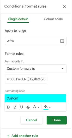
=ISBETWEEN($A2, DATE(2021, 3, 1), DATE(2021, 3, 14))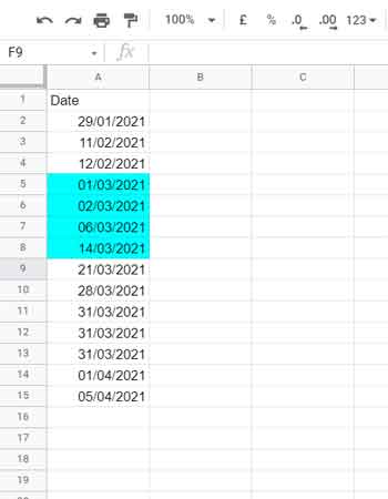

Dates highlighted with ISBETWEEN in Google Sheets

Explanation:

$A2 → the first cell in the date column (excluding the header).
DATE(2021, 3, 1) → start date.
DATE(2021, 3, 14) → end date.

The ISBETWEEN formula checks whether the date in cell A2 falls between 01/03/2021 and 14/03/2021. If TRUE, the conditional formatting rule highlights the cell.

To highlight the second fortnight, simply update the formula to use:

=ISBETWEEN($A2, DATE(2021, 3, 15), DATE(2021, 3, 28))

Apply to Range Setup

Under Apply to range, enter A2:A (or A2:Z if you want entire row highlighting).
Use $A2 in the formula so that the rule only tests values in column A, even if you apply it across multiple columns.

Conditional formatting sidebar with ISBETWEEN formula

This is a basic but practical example of the ISBETWEEN function in conditional formatting.

ISBETWEEN with Two Column Date Ranges

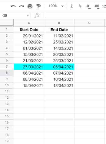
Now let’s look at a slightly advanced example where we have two columns:

Column A → Start Date
Column B → End Date

We want to highlight rows where today’s date falls within the range specified by columns A and B.

Row highlighting between two dates using ISBETWEEN

Formula:

=ISBETWEEN(TODAY(), $A2, $B2)

Explanation:

TODAY() → the current date (value being tested).
$A2 → start date.
$B2 → end date.

If today’s date lies between the values in columns A and B, the entire row is highlighted. You can replace TODAY() with any other date to test a different condition.

This demonstrates how flexible the ISBETWEEN function in conditional formatting can be when working with dynamic ranges.

You can also use ISBETWEEN to highlight rows where an actual value falls between a start and end column (similar to checking test results against their limits). For a detailed example, see Find Whether Test Results Fall within Their Limit in Google Sheets.

NOT with ISBETWEEN in Conditional Formatting

In the previous examples, TRUE values triggered highlighting. But what if you want to highlight values outside a specified range?

Example: You have time in column A and heart rate in column B. You want to highlight cases where the BPM is below 50 or above 100, assuming 50–100 BPM is the “normal” range.

Formula:

=AND(LEN($B2), NOT(ISBETWEEN($B2, 50, 100)))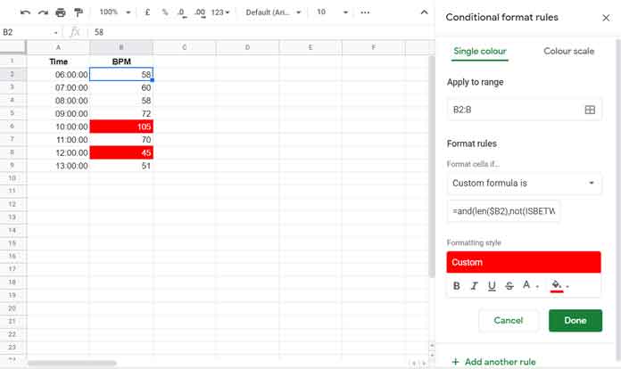

Highlighting values outside range with NOT and ISBETWEEN

Explanation:

ISBETWEEN($B2, 50, 100) → returns TRUE if BPM is between 50 and 100.
NOT(...) → flips the result, so values outside this range return TRUE.
LEN($B2) → prevents highlighting blank cells.
AND(...) → ensures both conditions are applied.

This highlights only the values that fall outside the safe range, which is useful for flagging exceptions.

Key Takeaways

The ISBETWEEN function in conditional formatting simplifies rules and makes them easier to read than using comparison operators.
It works for numbers, dates, and text.
You can use it with NOT, AND, or other functions to handle more complex scenarios.
It’s especially handy for highlighting date ranges, number ranges, and exceptions.

Conclusion

The ISBETWEEN function offers a cleaner and more intuitive way to build conditional formatting rules, especially when working with ranges of dates, numbers, or text. By combining it with functions like NOT and AND, you can handle both inclusion and exclusion scenarios with ease.

If you want to explore more ways to simplify and enhance your conditional formatting rules, check out the Ultimate Guide to Conditional Formatting in Google Sheets, where a wide range of related techniques are covered.