In this tutorial, you’ll create a monthly habit tracker in Google Sheets from scratch using checkboxes, formulas, conditional formatting, and automatic progress calculations. The tracker uses only built-in Google Sheets features—no Apps Script required.

By the end, you’ll have a clean, app-like habit tracker that automatically updates as you complete your habits.

Looking for a ready-to-use version instead? My free Google Sheets Habit Tracker Template includes 12 monthly trackers, yearly summaries, and works for any year—no setup required.

What You’ll Build in This Tutorial

A simple habit tracker only needs a list of habits and a few checkboxes. In this tutorial, you’ll build a more polished version with a dynamic calendar, automatic calculations, and a clean, app-like design.

You’ll learn how to:

• Set up the worksheet layout
• Create a dynamic monthly calendar
• Add and customize interactive checkboxes
• Apply formulas and conditional formatting
• Calculate habit completion percentages and monthly consistency

Step 1: Set Up the Worksheet

1. Open a new spreadsheet by visiting sheets.new.
2. Rename the spreadsheet to Habit Tracker (or any name you prefer).
3. Delete the rows below row 13 to keep the worksheet compact while building the tracker. This provides space for tracking 10 habits. You can always insert additional rows later if needed.
4. Insert 8 columns to the right of column Z so the sheet extends to column AH.
5. Set the following column widths:
   • Column A: 206 px
   • Columns B:AF: 28 px
   • Column AG: 120 px
   • Column AH: 50 px
6. Set the row heights:
   • Row 1: 45 px
   • Rows 2–13: 30 px
7. Select the entire worksheet, then set the font to Roboto and apply Middle align (vertical alignment) from the toolbar.

Note: The row heights and column widths used in this tutorial are important for achieving the intended layout. Changing them may affect the appearance of the checkboxes and conditional formatting in later steps.

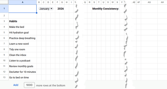
Step 2: Add the Month Selector and Habit List

Create the Month Selector

1. Merge cells B1:E1.
2. Create a drop-down list in the merged cell containing all 12 months (January through December) using Insert > Drop-down, then select a month (for example, January).
3. Merge cells F1:G1, then enter the current year (for example, 2026).

Add the Consistency Label

In X1, enter Monthly Consistency: and align it to the right.

Enter Sample Habits

1. Enter Habits in A3.
2. Enter the following sample habits in A4:A13 (replace them with your own if you prefer):

Make the bed
Hit hydration goal
Practice deep breathing
Learn a new word
Tidy one room
Clean the inbox
Listen to a podcast
Review monthly goals
Declutter for 10 minutes
Go to bed on time

Formatting: Use Bold text with a font size of 11 for the month selector (B1:E1), year (F1:G1), Monthly Consistency: label (X1), and Habits heading (A3).

Step 3: Create the Dynamic Calendar

Next, create a dynamic calendar that automatically updates whenever you change the selected month or year.

Enter the following formula in B3:

=LET(
  dt, DATE(F1, MONTH(B1&1), 1), 
  n, DAY(EOMONTH(dt, 0)), 
  SEQUENCE(1, n, dt)
)

The formula generates every date in the selected month. Because it returns full date values, we’ll format them to display only the day numbers.

Select B3:AF3, then choose Format > Number > Custom number format, enter dd, and click Apply.

Formula explanation

• dt stores the first date of the selected month and year.
• n calculates the number of days in that month.
• SEQUENCE returns n consecutive dates starting from dt.

Next, enter the following formula in B2 to display the abbreviated weekday names:

=ARRAYFORMULA(
  IF(
    B3:AF3, 
    CHOOSE(WEEKDAY(B3:AF3), "Su", "Mo", "Tu", "We", "Th", "Fr", "Sa"),
  )
)

Select the range B2:AF3, then center-align the contents horizontally.

Formula explanation

• WEEKDAY returns the weekday number for each date, where Sunday = 1 and Saturday = 7.
• CHOOSE converts those numbers into abbreviated weekday names such as Su, Mo, Tu, and so on.
• ARRAYFORMULA applies the formula to all dates returned in B3:AF3.

The calendar now updates automatically whenever you change the month or year.

Step 4: Add Checkboxes to Track Your Progress

In this step, we’ll add checkboxes to the habit tracker and apply the base formatting required for the final design.

1. Select the range B4:AF13.
2. Choose Insert > Tick box.
3. Set the font size to 26.
4. Center-align the cells horizontally.
5. Apply Light gray 2 as the fill color.

If you check a box at this stage, it displays the default check mark.

Step 5: Add the Conditional Formatting Rules

This step gives the habit tracker its clean, interactive appearance.

Apply the following four conditional formatting rules to the range B4:AF13 in the order shown below. The order is important because Google Sheets applies conditional formatting rules from top to bottom.

To add each rule, select the range B4:AF13, go to Format > Conditional formatting, choose Custom formula is, enter the formula, and then apply the specified formatting.

Rule 1: Blend Unused Cells into the Background

Custom formula

=OR($A4="", B$3="")

Formatting

• Fill color: White
• Text color: White

This rule makes cells blend into the background when either of the following conditions is met:

• The habit name in column A is blank.
• The corresponding calendar date is blank (for example, the 29th–31st in shorter months).

After applying this rule, cells for valid dates and non-empty habit rows remain light gray when unchecked, while all other cells blend into the white background.

Rule 2: Checked Boxes (Odd Rows)

Custom formula

=AND(B4, ISODD(ROW($A4)))

Formatting

• Fill color: #10B980
• Text color: #10B981

Using nearly identical fill and text colors hides the check mark while making checked cells appear as solid green blocks.

Rule 3: Checked Boxes (Even Rows)

Custom formula

=AND(B4, ISEVEN(ROW($A4)))

Formatting

• Fill color: #10B999
• Text color: #10B998

This uses a slightly different shade of green for alternating rows, making the tracker easier to scan.

Rule 4: Alternate Shading for the Tracking Area

Custom formula

=AND(ISODD(ROW($A4)), OR($A4<>"", B$3<>""))

Formatting

• Fill color: Light gray 3
• Text color: White

This rule applies alternating row shading to unchecked cells, making the tracker easier to read.

For a cleaner look, hide the worksheet gridlines by choosing View → Show → Gridlines and clearing the check mark.

After applying all four rules, checked boxes appear as green cells, unchecked boxes remain light gray, and cells outside the selected month’s dates and blank habit rows remain white, giving the tracker a clean, app-like appearance.

Step 6: Calculate Habit Progress

The layout is now complete. In this final step, we’ll calculate each habit’s completion percentage, display a progress bar, and summarize your overall monthly consistency.

Add the Progress Bars and Percentages

Enter the following formula in AG4:

=BYROW(
  B4:AF, 
  LAMBDA(r, LET(status, 
    COUNTIF(r, TRUE)/COUNTIF(B3:AF3, ">0"), 
    HSTACK(
      SPARKLINE(status, {"charttype", "bar"; "max", 1; "color1", "#2563EB"}), 
      status
    )
  ))
)

The formula returns the following:

• A sparkline progress bar in AG4:AG13.
• The corresponding completion percentage in AH4:AH13.

Select AH4:AH13, then choose Format > Number > Custom number format and enter:

0.0%;-0.0%;""

This custom number format displays percentages with one decimal place and hides empty cells.

Formula Explanation

• r represents each habit row in the range B4:AF.
• status stores the completion percentage by dividing the number of checked cells in the row by the number of valid calendar days in the selected month.
• SPARKLINE creates a horizontal progress bar based on the status value.
• HSTACK combines the progress bar and the completion percentage into two adjacent columns.
• BYROW applies the calculation to every habit row and spills the results automatically.

Add the Monthly Consistency Score

Merge Z1:AC1 then enter the following formula in the merged cell:

=AVERAGEIF(A4:A,"<>", AH4:AH)

This formula returns the average completion percentage across all listed habits.

Set the font size of the merged cell to 17.

Apply the same custom number format:

0.0%;-0.0%;""

How the Tracker Works

• Select a month from the drop-down list.
• In the checkbox area, click a cell to mark a habit as completed. You can also use the arrow keys to select a cell and press Spacebar to toggle the checkbox.
• The progress bars, completion percentages, and monthly consistency score update automatically.
• To mark a habit as incomplete, click the checkbox again or press Spacebar.

Note:

To avoid accidental errors while using the tracker, keep the following in mind:

• Don’t press the Delete key in the checkbox area. Doing so removes the underlying checkboxes.
• To mark a habit as complete or incomplete, click the cell or press Spacebar while it is selected.
• To check or uncheck multiple cells at once, select the range and press Spacebar once or twice.
• Before switching to a different month, uncheck all checked boxes. Otherwise, cells outside the selected month’s dates (such as the 29th–31st when switching to February) may still contain checked checkboxes, which can affect the progress calculations.

Frequently Asked Questions

Can I track more than 10 habits?

Yes. Click the Add button below the last row of the tracker and insert as many rows as you need. The formulas, conditional formatting, and checkboxes are copied automatically, so there’s no need to configure anything manually.

Can I use the tracker for any year?

Yes. Simply update the year in F1 and select a month from the drop-down list.

Why do I see “You may have clicked on a checkbox that is not visible”?

Cells for dates that don’t exist in the selected month and blank habit rows are intentionally formatted to blend into the background. Although the checkboxes are hidden from view, they still exist in those cells, so Google Sheets displays this message if you click them. You can safely select Cancel and continue using the tracker.

Can I turn this into a yearly habit tracker?

Yes. Simply duplicate the worksheet for each month and select the appropriate month from the drop-down list (January, February, and so on). This gives you a complete 12-month habit tracker.

If you’d also like an interactive yearly dashboard with automatic summaries and charts, you’ll need a few additional formulas. My Google Sheets Habit Tracker Template includes these features out of the box.

Can I customize the colors?

Yes. You can change the colors in the conditional formatting rules. However, keep the fill color and text color as slightly different shades of the same color. This hides the check mark while preserving the filled-cell effect.

Why is the monthly consistency greater than 100%?

The monthly consistency can exceed 100% if there are checked boxes in cells that are blended into the background. This usually happens when you switch to a shorter month (such as February) without first clearing the checkboxes for the 29th–31st, or when blank habit rows contain checked boxes.

To fix this issue, switch back to the previous month, clear all checked boxes, and then select the new month. To prevent it from happening again, always clear all checked boxes before changing the month and remove any unused habit rows.

Conclusion

You’ve now created a clean, automated monthly habit tracker in Google Sheets. It automatically generates the calendar, tracks completed habits, calculates completion percentages, and summarizes your monthly consistency using built-in Google Sheets features.

If you have any questions or run into any issues while building the tracker, feel free to ask in the comments below.

Looking for more ready-to-use spreadsheets? Browse my collection of Free Google Sheets Templates (Premium & Fully Automated) for additional templates that you can copy and customize.