This post explains how to create vertical and horizontal percentage progress bars in Google Sheets.
A percentage progress bar is a bar within a single cell that adjusts based on input values ranging from 0 to 100%. You can create such a bar in Google Sheets using either the SPARKLINE function or the REPT function.
The SPARKLINE function is the sole option for a vertical percentage progress bar, while for the horizontal version, both SPARKLINE and REPT can be employed.
The primary advantage of REPT over SPARKLINE lies in its ability to include text at the end point of the bar, indicating the total percentage achieved. However, it does come with a few drawbacks:
- Inflexibility with Length: REPT has a predefined length of 100%, and adjusting the cell size (column width) is necessary to accommodate it.
- Potential Inaccuracy: It may not provide 100% accuracy in depicting progress, as it employs a specific character to draw the bar.
- Vertical Limitation: REPT cannot be used to create a vertical progress bar.
Consider these factors when choosing between SPARKLINE and REPT for your percentage progress bar in Google Sheets.
Creating a Horizontal Percentage Progress Bar in Google Sheets
For example purposes, we will utilize the percentages in the cell range A2:A5, which are 25%, 100%, 50%, and 75%, respectively.
We will create a percentage progress bar for each of these values separately in the cell range C2:C5. Let’s begin with the first option, which involves using the SPARKLINE function.
In cell C2, enter the following formula and drag it down to cell C5:
=SPARKLINE(A2, {"charttype", "bar"; "color1", "green"; "max", 100%})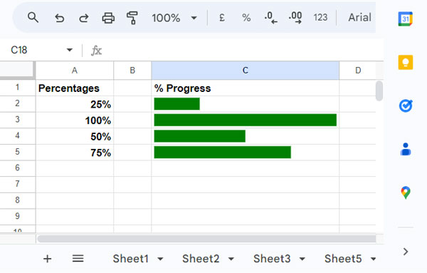
This will generate the chart in green, as specified by the “color1” option. You can replace “green” with “red” if you prefer a red color.
Suppose you want the percentage progress bar to display two colors: red below 50% and green above 50%. In that case, use an IF logical operation with the “color1” option as follows:
=SPARKLINE(A2, {"charttype", "bar"; "color1", IF(A2<=50%, "red", "green"); "max", 100%})This chart will automatically adjust based on the column width and row height.
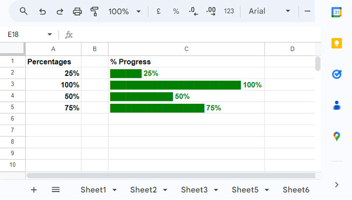
How to Add Text to My Horizontal Percentage Progress Bar in Google Sheets
The SPARKLINE function does not support the direct addition of text. If you wish to display text alongside the percentage progress, you’ll need to employ the REPT function method.
Follow these steps, keeping in mind that it has limitations regarding row height and column width flexibility.
- Begin by setting the percentage progress for the value in cell A2, initially set to 100% for ease of step-up.
- Enter the following formula in cell C2:
=REPT("█", A2*100/4)&TEXT(A2, " 0%") - Evaluate the length of the bar. If it meets your preferences, you can proceed without any adjustments to the formula.
- If you want to reduce the size, replace the
4in100/4with multiples of 2, such as 100/6 or 100/8. - If you want to increase the size, replace
100/4with100/2or simply use100.
Once set, match the column width to the size of the bar. Now you can replace the percentage value in cell A2 with the desired one (e.g., 25%) and drag down the formula as previously instructed.
This is the sole method to include text with a percentage progress bar in Google Sheets.
How Do I Change the Color of the Bar?
To change the color of the bar, navigate to the cell containing the REPT formula, click on “Text color” within the Google Sheets toolbar, and apply the color you desire.
Creating a Vertical Percentage Progress Bar in Google Sheets
For creating the horizontal percentage progress bar, we used the SPARKLINE bar chart option. Here, we will use the column option instead.
The following formula in cell C5 will create a vertical percentage progress bar using the percentage value in cell B5:
=SPARKLINE(B5, {"charttype", "column"; "ymin", 0%; "ymax", 100%; "color", "green"})It’s flexible and will adjust according to the row height and column width. I suggest increasing the row height and reducing the column width to see a genuine vertical percentage progress bar.
To conditionally adjust the color based on the 50% mark, as mentioned earlier, use an IF logical test within.
=SPARKLINE(B5, {"charttype", "column"; "ymin", 0%; "ymax", 100%; "color", IF(B5<=50%, "red", "green")})
Resources
The SPARKLINE function is widely used to create miniature charts in Google Sheets. The above is an example of one such use case.
In addition to creating percentage progress bars and other miniature charts, we can use the SPARKLINE function to generate GANTT charts in Google Sheets. Here are some tutorials that will help you advance in using this function in Google Sheets.


And sorry to bother you again, but is there any way to display the progress percentage at the right location?
I don’t need the fancy border or padding, but I’m just curious to know if it’s possible without using Apps Script?
Hi, Trang,
It’s not possible with the SPARKLINE. But I have a new solution based on the other formula.
I hope you will like it. See ‘Sheet3’ in my example Sheet. I have added more customization to the progress bar. You can change the color, size, style by changing the font color, size, and font.
Prashanth,
Thank you for taking the time to help me. I don’t know that I can do so many things with the Sparkline function.
Thank you, Prashanth. I’ve been getting into Google Sheets lately and you always have the answer to many questions I have.
I’m happy with the result I’ve got from using the Sparkline function to make the progress bar, but I’ve come across the dashboard of the Samsung health app and like the design of the daily timeline there.
Basically, every day starts from 12am and ends at 12pm. It is visualized as a simple straight line. NOW is represented by a dot and its location on the line indicates the approximate time of day.
Do you have any idea how to replicate this design? I know that it certainly wasn’t designed in Google Sheets, but I’m still curious about that.
Hi, Trang,
There is no such chart available in Google Sheets. Here is an alternative but NOW is not represented by a dot or any other mark. That’s a drawback.
Steps:
Enter the time 00:00 in cell A2 and 01:00 in A3. Drag down until A26.
In the range B2:B26, enter the number of steps in each cell based on the time of the left (column A).
Use this formula in cell D1.
=sparkline(B2:B26,{"charttype","column";"color","blue";"lowcolor","red";"highcolor","green";
"firstcolor","black";"lastcolor","black";"negcolor","blue";"empty","zero";
"nan","convert";"axis",TRUE;"axiscolor","cyan";"ymin",0;"ymax",max(B2:B26);
"rtl",FALSE})
This formula uses the SPARKLINE column chart. You can find the details of this formula use below.
Sparkline Column Chart Options in Google Sheets.
This is exactly what I was looking for! Any way to have the progress bar that is generated shrink to fit? I have it so that the cell holding the formula for the progress bar is merged across 3 cells and for a progress bar that is supposed to reflect a little over 50% progress, it spans 3/4 of the 3 cells. Visually this is pretty off. Any way to fix this?
Hi, Derek,
Sorry for the late reply. You can do that by dividing the % by ‘n’. I have included my example sheet and demonstrated the shrinking in ‘Sheet3’. In that, the ‘n’ is 4.
Fantastic hack! Thank you!
Thank you! What a creative and skilled solution. The explanation was clear too. I’m trying to display a progress bar for my custom goals and this worked perfectly!
Hi, would like to know how you did the conditional formatting, thanks!
It’s simple.
Select the cell E2 and then apply the following formula in the conditional formatting custom rule as below.
Format > Conditional Formatting >Custom formula is;
In this filed apply the below formula.
=and(C12>0,C12<20)This formula would highlight the cell E2 if the value in cell C12 is in between 0 and 20. Add multiple rules similarly. In each rule use different colors.
Thanks
Great. Thanks
SHARING THE SHEET WOULD HAVE MADE MUCH MORE SENSE
Hi Amged Osman ,
Welcome!
Below is the link to the Percentage Progress Bar in Google Sheets.
Please feel free to make a copy from the file menu for complete access.
https://goo.gl/GEsSDv
Thanks.