We can use the GETPIVOTDATA function in Google Sheets to extract multiple aggregated values and create an array or range. This is a valuable technique since such data can be utilized to generate multiple charts from a single Pivot Table.

Certainly, FILTER or QUERY can be employed to obtain the desired value from a Pivot Table. However, these methods have two drawbacks:

• Pivot Table movement: When you move the Pivot Table, you may need to edit the Pivot Table ranges used in the formula.
• Source data changes: When you edit the source data, the Pivot Table may expand or shrink. So the columns or rows used for filtering may need to be adjusted. Additionally, these functions require expertise in crafting criteria-based filtering.

The GETPIVOTDATA function is designed to return a single aggregated value, and using the ARRAYFORMULA function with it won’t be helpful. To obtain multiple values with GETPIVOTDATA, one should use one of the LAMBDA helper functions with it.

Below, we will explore several examples of using the MAP Lambda Helper function with GETPIVOTDATA in Google Sheets to return an array or range.

Given the diversity of Pivot Table settings, such as multiple row grouping, row and column grouping, multiple aggregations, and more, a single example may not cover all techniques.

Let’s unlock the potential of GETPIVOTDATA arrays in Google Sheets with a few illustrative examples!

Fictitious Data for Testing GETPIVOTDATA Array Formulas

The sample data consists of three columns: Player, Game, and Score. This dataset is suitable for testing multiple row grouping and row & column grouping.

Player	Game	Score
John	Formula Frenzy	5
John	Formula Frenzy	5
John	Data Daze	8
John	Data Daze	7
Emily	Formula Frenzy	4
Emily	Formula Frenzy	3
Emily	Data Daze	9
Emily	Data Daze	6

There are two players (John and Emily) and two games (Formula Frenzy and Data Daze). The first two columns in the table contain this data. Each player participated in each game twice, and you can find their scores in the third column.

We will create a Pivot Table from this dataset to test GETPIVOTDATA array formulas in Google Sheets. To access the sample data and all the formula examples, copy the sample sheet by clicking the button below.

Sample Sheet

Pivot Table with Multiple Row Grouping and GETPIVOTDATA Array Formulas

To test the GETPIVOTDATA function with multiple values, the first step is to create a Pivot Table report. Follow the steps below to create a Pivot Table from the provided data with two-row grouping:

Creating a Pivot Table

1. Assume the table is in the cell range A1:C9 in “Sheet1.”
2. Move to cell A11.
3. Click on Insert > Pivot Table.
4. In the “Data range” field, enter the range A1:C9.
5. Select “Existing sheet” since we are inserting the Pivot Table in the existing sheet that contains the source data.
6. Enter A11 in the provided field.
7. Click “Create.”

Upon completing the above steps, Sheets will insert the layout of the Pivot Table and open the Pivot Table Editor panel on the sidebar.

1. Drag and drop the fields “Player” and then “Game” below Rows.
2. Drag and drop the field “Score” under Values twice. Set “Summarize by” SUM and AVERAGE.
3. With these steps, the Pivot Table is now created. Now, let’s explore the GETPIVOTDATA array formula to retrieve multiple values from this Pivot Table report.

Combining GETPIVOTDATA with MAP and LAMBDA in Google Sheets

Fetching Multiple Data Points from a Pivot Table:

• Syntax of GETPIVOTDATA:

GETPIVOTDATA(value_name, any_pivot_table_cell, [original_column, …], [pivot_item, …])

• Key Points:
  • The GETPIVOTDATA function extracts specific data from a Pivot Table.
  • It cannot directly return multiple values.
  • MAP and LAMBDA expand its capabilities to retrieve multiple results.

Example Scenario # 1 (Row Grouping)

(Refer to Sheet1 in the Sample Sheet above)

Retrieve the average scores of Emily and John in the game “Formula Frenzy.”

To achieve this, begin by creating a table as illustrated below in the range E1:G3:

Player	Game	AVERAGE of Score
Emily	Formula Frenzy
John	Formula Frenzy

Note that the GETPIVOTDATA function does not support specifying more than one pivot_item directly, as demonstrated below:

=GETPIVOTDATA(G1, A11, E1, E2:E3, F1, F2:F3) // incorrect formula!

Since direct specification of an array within GETPIVOTDATA is not supported, we utilize the MAP function to iterate over each value in the array, thereby enabling the retrieval of multiple results.

To obtain the average score for both players, enter the following array formula in cell G2, which will spill to G3:

=MAP(E2:E3, F2:F3, LAMBDA(a, b, GETPIVOTDATA(G1, A11, E1, a, F1, b)))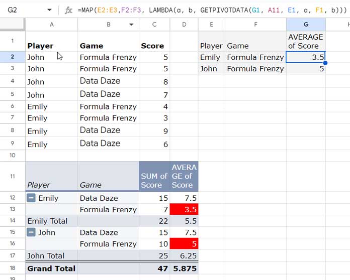

Formula Breakdown

Note: The explanation below delves into the formula’s finer details, including the use of MAP and LAMBDA functions. If you’re new to these concepts, feel free to skip this section and proceed directly to the next example.

MAP Function:

MAP(array1, [array2, …], LAMBDA([name, …], formula_expression))

The MAP function applies a specified LAMBDA function to each corresponding pair of elements in two arrays and returns an array of results. In this case:

• array1: E2:E3 (Player names – Emily and John)
• array2: F2:F3 (Game names – Formula Frenzy)

LAMBDA Function:

=LAMBDA(a, b, GETPIVOTDATA(G1, A11, E1, a, F1, b))

The LAMBDA function defines an anonymous function that takes two arguments (a and b) and returns the result of the enclosed expression, which is a GETPIVOTDATA function in this case.

GETPIVOTDATA Argument Explanations:

• value_name: G1 (“AVERAGE of Score”)
• any_pivot_table_cell: A11 (references a cell within the Pivot Table)
• original_column: E1 (“Player”)
• pivot_item: a (each player from the result table)
• original_column: F1 (“Game”)
• pivot_item: b (each game from the result table)

Example Scenario # 2 (Row Grouping)

(Refer to Sheet2 in the Sample Sheet above)

To retrieve both “AVERAGE of Score” and “SUM of Score” in the array formula, follow these steps:

1. Enter “SUM of Score” in cell H1.
2. Use this nested MAP formula in cell G2:

=MAP(G1:H1, LAMBDA(x, MAP(E2:E3, F2:F3, LAMBDA(a, b, GETPIVOTDATA(x, A11, E1, a, F1, b)))))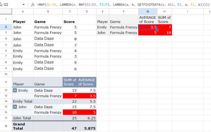

Explanation:

Outer MAP Function:

• Iterates over each value in the value_name array (G1:H1), containing “AVERAGE of Score” and “SUM of Score”.
• Applies the inner MAP function for each value_name.

Inner MAP Function:

• Iterates over each combination of pivot_items, where player names are taken from E2:E3 and game names from F2:F3.
• Retrieves the specified value (AVERAGE or SUM) using GETPIVOTDATA for each player and game combination.

LAMBDA Function (within inner MAP):

• Takes player and game as arguments.
• Uses GETPIVOTDATA to retrieve the specified value based on the current value_name.

Pivot Table with Row & Column Grouping and GETPIVOTDATA Array Formulas

In this case, the Pivot Table layout has been altered. The “Player” field is grouped, and the “Game” field is pivoted.

Example Scenario # 1 (Row and Column Grouping)

(Refer to Sheet3 in the Sample Sheet above)

Pivot Table Structure:

• Drag and drop the “Game” field under Columns and the “Player” field under Rows in the Pivot Table editor.
• Place “Score” under Values and summarize using the AVERAGE function.

Creating the Data Table:

• Establish a table in the range E1:G3 as follows:

	Data Daze	Formula Frenzy
Emily
John

Enter the following GETPIVOTDATA formula in cell F2 to fetch multiple aggregated values from the Pivot Table:

=MAP(F1:G1, LAMBDA(c, MAP(E2:E3, LAMBDA(r, GETPIVOTDATA(A11, A11, "Player", r, "Game", c)))))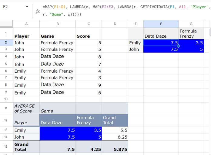

Here, I’ll keep the formula explanation brief, assuming familiarity with the nested MAP function from our previous example.

Breakdown:

• Outer MAP: Iterates over columns in F1:G1 (game names).
• Inner MAP: Iterates over rows in E2:E3 (player names).
• GETPIVOTDATA: Retrieves data from a Pivot Table:
  • First A11 (value_name): Specifies the name of the value to extract (e.g., “AVERAGE of Score”).
  • Second A11 (any_pivot_table_cell): References a cell within the Pivot Table (likely top-left).
  • “Player” (original_column): Field to retrieve data from.
  • r (pivot_item): Current row value (player name) from the inner MAP.
  • “Game” (original_column): Field to filter by.
  • c (pivot_item): Current column value (game name) from the outer MAP.

Result: The formula populates the table with average scores for each player-game combination, extracted dynamically from the Pivot Table.

Example Scenario # 2 (Row and Column Grouping)

(Refer to Sheet4 in the Sample Sheet above)

This time, there’s an additional change in the Pivot Table. In the example above, “Player” is grouped, and “Game” is pivoted with the aggregation set to AVERAGE.

Now, for this scenario, we’ll use the same Pivot Table but with an additional aggregation, which is SUM.

In short, add “Player” under Rows, “Game” under Columns, and place “Score” twice under Values.

Next, create the following table in cell E1:H3 for use in the GETPIVOTDATA array formula.

		AVERAGE of Score	SUM of Score
Emily	Formula Frenzy
John	Data Daze

Formula (in cell G2):

=MAP(G1:H1, LAMBDA(x, MAP(E2:E3, F2:F3, LAMBDA(a, b, GETPIVOTDATA(x, A11, "Player", a, "Game", b)))))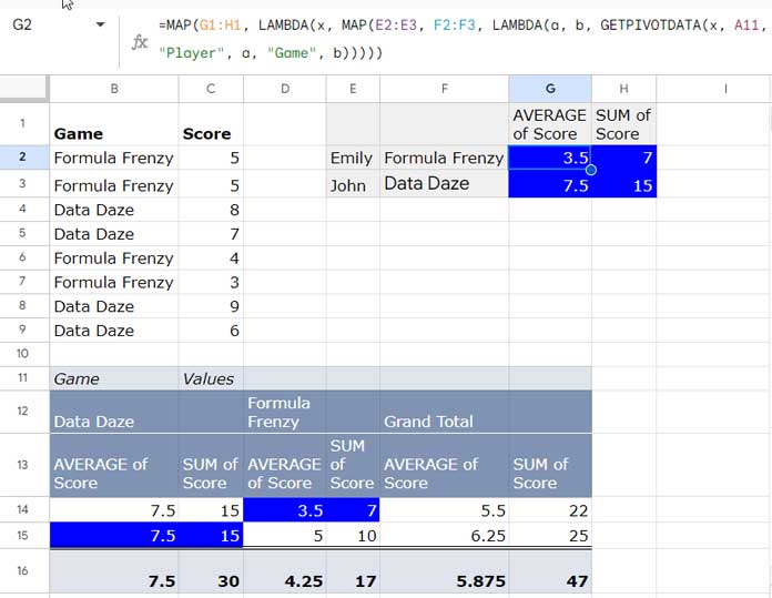

Formula Breakdown

• Outer MAP: Iterates over columns in G1:H1 (representing AVERAGE and SUM).
• Inner MAP: Iterates over rows in E2:E3 (players) and columns in F2:F3 (games).
• GETPIVOTDATA: Retrieves data from the Pivot Table:
  • x (value_name): Current column value from the outer MAP (AVERAGE or SUM).
  • A11 (any_pivot_table_cell): References a cell within the Pivot Table (likely top-left).
  • “Player” (original_column): Field to retrieve data from.
  • a (pivot_item): Current row value from the inner MAP (player name).
  • “Game” (original_column): Field to filter by.
  • b (pivot_item): Current column value from the inner MAP (game name).

The formula dynamically populates the table with both average scores and the sum of scores for each player-game combination, extracted from the Pivot Table based on the specified aggregation.

GETPIVOTDATA Array and Charting in Google Sheets

Utilizing the GETPIVOTDATA function to return an array value in Google Sheets offers specific advantages.

When creating charts from a Pivot Table, you might need to exclude the TOTAL/GRAND TOTAL rows and columns, a step you may prefer to avoid.

In such cases, the combination of GETPIVOTDATA and MAP can be employed to fetch the required values from the Pivot Table and facilitate chart plotting.

For instance, refer to the example scenario #1 under “Pivot Table with Row & Column Grouping and GETPIVOTDATA Array Formulas.” You can use the resulting table to create a column or bar chart.

Additional Tips

When generating the resulting table, you can employ the UNIQUE function in the source data to dynamically obtain the original_column values.

For Player names in the given examples, use the following formula:

=UNIQUE(A2:A9)

Similarly, to obtain unique game names, use the formula:

=UNIQUE(B2:B9)

This approach adds dynamism to the GETPIVOTDATA array formula.

Explore additional functions like VSTACK, HSTACK, TOCOL, and TOROW as they can enhance flexibility when working with the resulting table.

Resources:

• Create Pivot Charts in Google Sheets.
• Filter Multiple Values in the Pivot Table in Google Sheets.