Unlike Microsoft Excel, Google Sheets does not have a dedicated “PivotChart” menu option. Instead, you must first create a pivot table and then generate a chart from it, just like a regular graph.
Introduction to Pivot Charts in Google Sheets
Charts are graphical representations of data, and pivot charts are no exception. However, instead of using raw data, pivot charts are created from a pivot table.
Pivot tables help summarize large datasets without requiring complex formulas. A pivot chart visually represents the pivot table, allowing you to identify trends, comparisons, and patterns easily. Mastering pivot charts in Google Sheets is essential for creating dynamic and interactive dashboards.
How to Create Pivot Charts in Google Sheets
Pivot charts cannot be created directly from a pivot table if it contains subtotal and grand total rows. The solution is to duplicate the pivot table and remove those total rows.
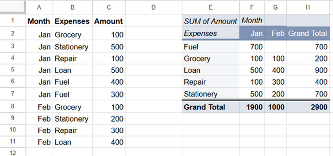
In this tutorial, we will use the following sample data:
| Month | Expenses | Amount |
| Jan | Grocery | 100 |
| Jan | Stationery | 500 |
| Jan | Repair | 100 |
| Jan | Loan | 500 |
| Jan | Fuel | 400 |
| Jan | Fuel | 300 |
| Feb | Grocery | 100 |
| Feb | Stationery | 200 |
| Feb | Repair | 300 |
| Feb | Loan | 400 |
Step 1: Creating the Pivot Table
- Select the range A1:C (your dataset).
- Click Insert > Pivot table.
- In the window that appears, select Existing Sheet and choose an empty cell (e.g., E1).
- Click Create.
- In the Pivot Table Editor (sidebar), set up the pivot table as follows:
- Drag Expenses under Rows.
- Drag Month under Columns.
- Drag Amount under Values.
- Add Expenses under Filters and apply the filter:
- Select Filter by Condition > Is Not Equal To.
- Enter the formula:
=""
This will create a structured pivot table.
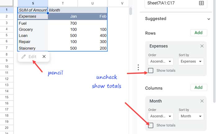
Step 2: Duplicating the Pivot Table
To create a pivot chart, we need to work with a modified version of the pivot table.
- Copy the pivot table from E1.
- Paste it into S1 (in a distant column to allow for future expansion).
- Remove grand total row and column:
- Click the Edit (pencil) icon on the new pivot table.
- Uncheck “Show Totals” in the Pivot Editor.
Step 3: Adding Dummy Field Labels
Google Sheets allows dynamic row expansion in charts but not dynamic column expansion. To ensure our pivot chart remains adaptable, add dummy headers before creating the chart:
- Enter placeholder labels in V2 and M2 (or more, depending on expected future columns). We will delete them later.
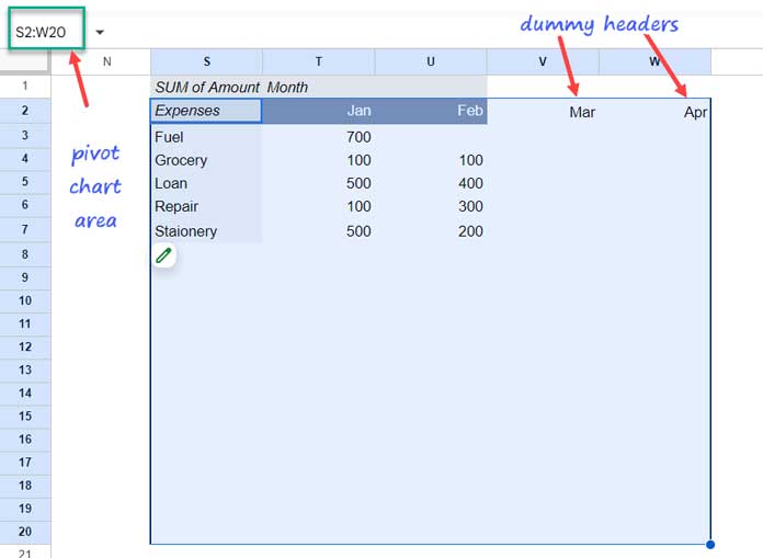
Now, the dataset is ready for chart creation.
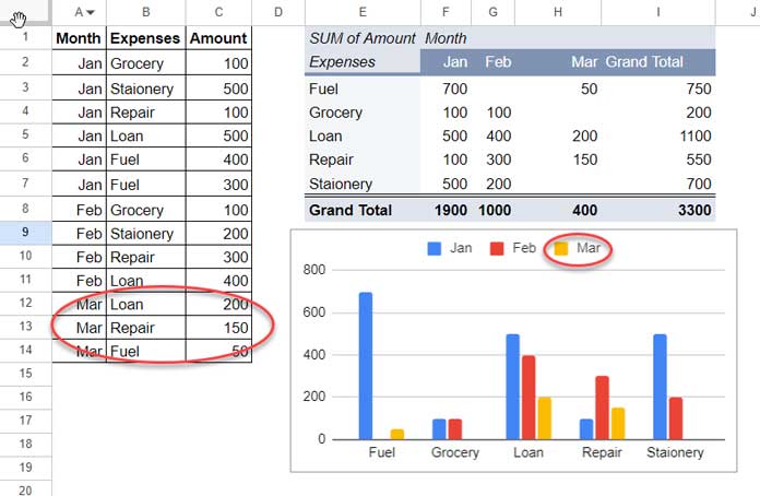
Step 4: Creating the Pivot Chart
- Select the range S2:W20 (including extra rows and columns for future data).
- Click Insert > Chart.
- In the Chart Editor, check “Row 2 as headers”.
- Remove the dummy headers after confirming the chart is working.
- Add new data in A2:C—the pivot chart will update automatically!
Now you have a fully dynamic pivot chart in Google Sheets!
FAQs
Can I hide the duplicate pivot table?
Yes! Right-click the column letter and select Hide column to keep your sheet clean.
⚠️ You may see a “Data in hidden columns is excluded from the chart” warning. Click “Include Hidden/Filtered Data” in the Chart Editor under the Setup tab.
What chart types are supported in Google Sheets’ pivot charts?
There are no restrictions! You can use any chart type, including:
- Column Chart
- Bar Chart
- Pie Chart
- Line Chart
- Scatter Chart
Can I create a pivot chart without a duplicate pivot table?
Yes, you can use the QUERY function to generate a pivot table dynamically. However, this method requires familiarity with the QUERY function.


