


This is an introductory post on the VLOOKUP and HLOOKUP functions in Google Sheets, featuring basic examples and links to detailed tutorials on this blog.
The essence of this post is to help you comprehend the significance of vertical and horizontal lookups in Google Sheets.
For spreadsheet users engaged in serious data entry, knowing how to use VLOOKUP and HLOOKUP is a source of pride. Recently, XLOOKUP has gained prominence in this context.
I’ve emphasized VLOOKUP in this post. Begin by understanding how to use VLOOKUP in Google Docs Spreadsheet, and then proceed similarly with HLOOKUP. As always, I’ve aimed to keep this tutorial as simple as possible.
What Is VLOOKUP?
If your data is organized in rows, you can employ the VLOOKUP function to search for a specific value.
The function utilizes a search key, scanning down the first column of the lookup range (table) and retrieving a value from the specified column or columns.
It identifies the initial instance of the search key in the first column of the range and delivers the corresponding result from the same row.
When employing numbers, dates, datetime, or time as the search key, if no exact match is found, the formula will return the value less than or equal to the search key—provided the data is sorted A-Z.
What Is HLOOKUP?
If your data is organized in columns, you can utilize the HLOOKUP function to search for a specific value.
Unlike VLOOKUP, HLOOKUP searches for the key in the first row and returns the value from the corresponding columns. All other features remain the same.
VLOOKUP Use Case: Basic Example to Understand the Function
Syntax:
=VLOOKUP(search_key, range, index, [is_sorted])Arguments:
search_key: The value to search.range: The range to search.index: The column index, e.g., 5.is_sorted: Choose TRUE (sorted) or FALSE (unsorted).
Before we start with the formula, type the following data in a Google Docs Spreadsheet in the range A1:D6.
| Item Code | Description | Unit Price (Ton) | Markup |
| W-220 | White Pebbles 20 mm | 750.00 | 22% |
| Bl-220 | Black Pebbles 20 mm | 800.00 | 24% |
| W-240 | White Pebbles 40 mm | 700.00 | 26% |
| Bl-240 | Black Pebbles 40 mm | 750.00 | 22% |
| Br-240 | Brown Pebbles 40 mm | 800.00 | 30% |
Problem:
Find the retail price of the item “White Pebbles 40 mm” by searching for the item code “W-240” in the range.
To find the retail price, we need to first Lookup the unit price and markup percentage of “W-240” and apply the following formula:
Retail Price=Unit Rate×(1+Markup Percentage)
We will use one VLOOKUP to extract the unit rate and another VLOOKUP to extract the markup percentage.
The following VLOOKUP will return the unit rate from the table:
=VLOOKUP("W-240", A1:D6, 3, false)Where:
search_key: “W-240”range: A1:D6index: 3 (to return the result from the third column)is_sorted: false
To return the markup percentage, we can use the same formula but with index # 4, and here it is:
=VLOOKUP("W-240", A1:D6, 4, false)Now let’s apply the formula to calculate the retail price, and here it is:
=VLOOKUP("W-240", A1:D6, 3, false)*(1+VLOOKUP("W-240", A1:D6, 4, false))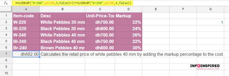
I hope the above example helps you understand when and where to use the VLOOKUP function in Google Sheets. For detailed information on the function, please refer to the following guides.
Mastering VLOOKUP: In-Depth Guides and Tips for Success
Core Function:
Supporting Tutorials:
- How to Use VLOOKUP with Multiple Criteria in Google Sheets [Solved]
- Multiple Values Using Vlookup in Google Sheets is Possible [How to]
- How to Use Vlookup to Return An Array Result in Google Sheets
- Dynamic Index Column in Vlookup in Google Sheets
Improve the Level:
- How to Perform Two-way Lookup Using Vlookup in Google Sheets
- Reverse Vlookup Examples in Google Sheets [Formula Options]
- How to Vlookup Importrange in Google Sheets [Formula Examples]
- Vlookup Last Record in Each Group in Google Sheets
- Nested Vlookup in Google Sheets
- Common Errors in Vlookup in Google Sheets
- Vlookup and Combine Values in Google Sheets
- Wildcards in Vlookup Search Range in Google Sheets
HLOOKUP Use Case: Basic Example to Understand the Function
Syntax:
HLOOKUP(search_key, range, index, [is_sorted])Arguments:
search_key: The value to search.range: The range to search.index: The row index, e.g., 3.is_sorted: Choose TRUE (sorted) or FALSE (unsorted).
Now, you can grasp the utilization of HLOOKUP through the following example and subsequent links to detailed tutorials.
First, copy and paste the above data as follows into the range A14:F17 using the Transpose function in your Google Sheets.

Now that the data is arranged in columns, let’s address the same problem that we solved using VLOOKUP here.
We are using HLOOKUP because the data is transposed, and we want to search the first row and return values from the third and fourth rows in the found column.
The following HLOOKUP will return the unit rate from the table:
=HLOOKUP("W-240", A14:F17, 3, false)Where:
search_key: “W-240”range: A14:F17index: 3 (to return the result from the third row)is_sorted: false
To return the markup percentage, we can use the same formula but with index # 4, and here it is:
=HLOOKUP("W-240", A14:F17, 4, false)To get the retail price, let’s apply the formula: Retail Price=Unit Rate×(1+Markup Percentage)
=HLOOKUP("W-240", A14:F17, 3, false)*(1+HLOOKUP("W-240", A14:F17, 4, false))Mastering HLOOKUP: In-Depth Guides and Tips for Success
Core Function:
Supporting Tutorials:
- How to Return an Entire Column in Hlookup in Google Sheets
- How to Do a Reverse Hlookup in Google Sheets
- How to Use Multiple Conditions in Hlookup in Google Sheets
Improve the Level:
- Vlookup and Hlookup Combination In Google Sheets
- Hlookup to Search Entire Table and Find the Header in Google Sheets
- Move Single Column to Multiple Columns Using Hlookup in Google Sheets
Conclusion
The purpose of this tutorial is to help you comprehend the VLOOKUP and HLOOKUP functions. Both of these functions require detailed study, which cannot be fully covered in a single tutorial.
To further your understanding, I have included links to several advanced lookup tutorials in this post. Additionally, you can discover more by using the search feature within this blog.
Thank you for reading.
Hi,
Is it possible to import every Nth Cell from another Sheet?
I am trying to import every 6th cell from Column C. I’ve tried doing this but I keep ending up with the imported data appearing every 6 rows.
I then tried to sort the range this compiled the data but also alphabetized it which I don’t want. Thanks!
Hi, Abi,
You can check this guide – Import Every Nth Row in Google Sheets Using Query or Filter (Same File).
Thank you! 😀
I’m trying to use Vlookup to pull a value from a different tab by referencing that tab from the matching string in the cell above it (attempting to use the Indirect function).
My formula looks like this:
=VLOOKUP($B5,'(=INDIRECT("C3"))'!$O$3:$S$6,5,false)Where C3 contains a text string which has the same name as the TAB I’m trying to pull the data from. It works fine when I simply write the name of the tab in the formula ie
=VLOOKUP($B5,'Sheet1'!$O$3:$S$6,5,false)but this is tedious for copying the formula across cells, because each cell is pulling data from a separate tab (with different sheet name of course). Hope that is clear.Suggestions?
Hi, Steve,
As per your example, the use of Indirect in Vlookup must be as follows.
=VLOOKUP($B5,INDIRECT("'"&C3&"'!"&"$O$3:$S$6"),5,false)Best,