We can use a dynamic formula to sum the last value in a column across multiple sheets within a file in Google Sheets. The generic formula is as follows:
Generic Formula:
=ArrayFormula(LET(
   range, HSTACK(range1, range2, ...),
   lv, BYCOL(range, LAMBDA(c, XLOOKUP(TRUE, ISNUMBER(c), c, , 0, -1))),
   SUM(lv)
))range1: the column to test and extract the last number to include in the summation.range2, …: additional columns to test and extract the last number to include in the summation.
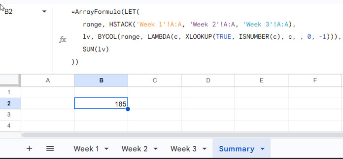
For example, to sum the last value in column A across multiple sheets, namely, in the range ‘Week 1’!A:A, ‘Week 2’!A:A, ‘Week 3’!A:A, we can use the following formula:
=ArrayFormula(LET(
   range, HSTACK('Week 1'!A:A, 'Week 2'!A:A, 'Week 3'!A:A),
   lv, BYCOL(range, LAMBDA(c, XLOOKUP(TRUE, ISNUMBER(c), c, , 0, -1))),
   SUM(lv)
))
This formula extracts and sums the last number in column A in the “Week 1,” “Week 2,” and “Week 3” sheets.
Here are some of the key features of the formula:
range1, range2, …can represent different columns in various sheets. For example, you can use column A in one sheet and column B in another.range1, range2, …can also denote different columns from the same sheet. For instance, you can use columns A and B from the same sheet.
Summing the Last Value in a Column Across Multiple Sheets: Formula Breakdown
The formula makes use of the LET function to define named value expressions. Let’s start by understanding this function.
Syntax:
LET(name1, value_expression1, [name2, …], [value_expression2, …], formula_expression)The assigned names in the formula are ‘name1’ and ‘name2’, represented as ‘range’ and ‘lv’, respectively.
- ‘range’ is:
HSTACK('Week 1'!A:A, 'Week 2'!A:A, 'Week 3'!A:A)This component combines values in column A from three different sheets (‘Week 1’, ‘Week 2’, and ‘Week 3’) horizontally, creating a unified range by stacking the columns.
- ‘lv’ is:
BYCOL(range, LAMBDA(c, XLOOKUP(TRUE, ISNUMBER(c), c, , 0, -1)))This part utilizes the BYCOL function in conjunction with a lambda function (anonymous function) to perform an operation column-wise. The lambda function, specifically XLOOKUP(TRUE, ISNUMBER(c), c, , 0, -1), searches for the last numeric value in each column, resulting in an array containing the last values from each column.
Related: Extract Last Values from Each Column in Google Sheets
The formula expression in the formula is:
SUM(lv)The SUM function is then applied to add up all the last values obtained from each column, providing the overall sum of the last values across the specified sheets.
Note: The formula uses the ISNUMBER function within the lambda function, which requires the ArrayFormula wrapper when using a range reference. This ensures that the formula is applied to the entire range of data rather than just a single cell.
In summary, the formula combines data from specific columns in different sheets, extracts the last numeric value from each column using the XLOOKUP function within a lambda function, and then calculates the sum of these last values across the specified sheets.
The use of LET enhances the readability and flexibility of the formula.
Summing Last Values in a Column Across Multiple Sheets with INDIRECT
This is an advanced tip that adds flexibility to the formula.
In the provided formula, the range to extract values is specified within the HSTACK as follows:
HSTACK('Week 1'!A:A, 'Week 2'!A:A, 'Week 3'!A:A)However, some users may prefer not to enter sheet names in the formula. This is where the INDIRECT function becomes useful.
Assuming you have sheet names within the range A2:A4 as follows:
| Week 1!A:A |
| Week 2!A:A |
| Week 3!A:A |
(Note: Do not enter an apostrophe with sheet names, for example, ‘Week 1’; it is not required.)
Replace the HSTACK('Week 1'!A:A, 'Week 2'!A:A, 'Week 3'!A:A) with the following formula:
REDUCE(TOROW(,1), A2:A4, LAMBDA(a, v, HSTACK(a, INDIRECT(v))))The formula to sum the last value in a column across multiple sheets by indirectly referencing a list of ranges will be as follows:
=ArrayFormula(LET(
   range, REDUCE(TOROW(,1), A2:A4, LAMBDA(a, v, HSTACK(a, INDIRECT(v)))),
   lv, BYCOL(range, LAMBDA(c, XLOOKUP(TRUE, ISNUMBER(c), c,, 0, -1))),
   SUM(lv)
))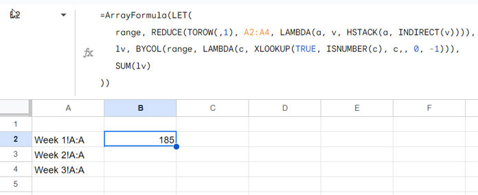
It’s important to note that the INDIRECT function in Google Sheets cannot handle multiple indirect ranges at once. Therefore, the REDUCE function is utilized to iterate over each value in the list (A2:A4).
For further details, refer to the tutorial on dynamically combining multiple sheets horizontally in Google Sheets, specifically the last part titled “Combine Multiple Sheets Horizontally by Referring to Sheet Names in a Range.”
Resources
Searching for Similar Formulas in Google Sheets? Here you have them!
- How to Find the Last Value in Each Row in Google Sheets
- How to Return First Non-blank Value in A Row or Column
- XMATCH First or Last Non-Blank Cell in Google Sheets
- Find the Cell Address of a Last Used Cell in Google Sheets
- Find the Last Entry of Each Item from the Date in Google Sheets
- Find the Average of the Last N Values in Google Sheets
- How to Find the Last Matching Value in Google Sheets
- How to Lookup First and Last Values in a Row in Google Sheets
- Lookup Last Partial Occurrence in a List in Google Sheets


