Google Sheets: Filter Rows with Furthest Data in Each Category

This tutorial explores advanced filtering techniques in Google Sheets, specifically focusing on filtering rows with the furthest data within each category.

We will apply the formula to an age analysis report (mockup data) that includes Customer Name and Inv. No. in columns A and B, along with the aging of invoices in columns C to G (Current, 30-60 days, 60-90 days, 90-120 days, and >120 days).

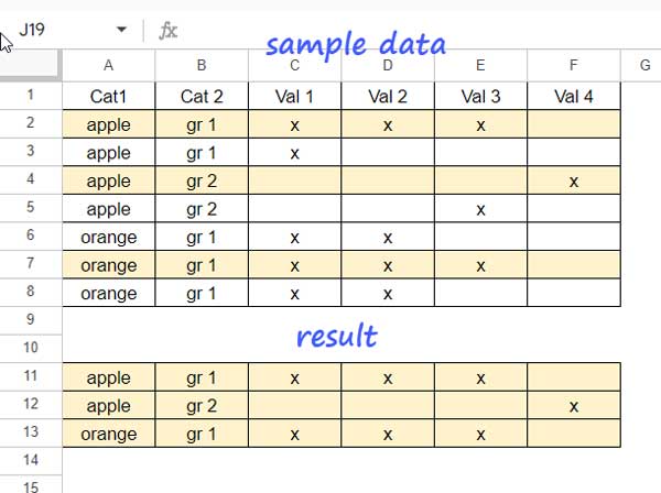
Sample Data:

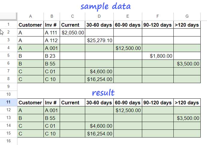
Category-wise filtering data with furthest data point in Google Sheets

The goal is to filter the furthest data, namely the invoice amount, within each category (customer).

As per the sample data, Customer A (category) has three pending invoices aging in the current (C), 30-60 days (D), and 60-90 days (E). The formula will filter the rows with the furthest entry, which, in this case, is row #4 containing the amount under 60-90 days.

The formula filters rows with the furthest data entry in each category (Customer), applying this filtering across all categories present. In short, it’s a category-wise filtering approach.

How to Filter Rows with Furthest Data in Each Category in Google Sheets

You can utilize the following formula to filter records with the furthest data in Google Sheets. Please remember to replace the range A2:G8 with your specific data range, excluding the header row.

=ArrayFormula(LET(
   table, A2:G8, 
   maxx, BYROW(table, LAMBDA(r, XMATCH(TRUE, r<>"", 0, -1))), 
   srtA, SORT(HSTACK(table, maxx), 1, 1, COLUMNS(table)+1, 0), 
   srtB, SORTN(srtA, 9^9, 2, CHOOSECOLS(srtA, 1), 1), 
   combine, TRANSPOSE(QUERY(TRANSPOSE(CHOOSECOLS(srtB, {1, COLUMNS(table)+1})),,9^9)), 
   fnl, XMATCH(TRANSPOSE(QUERY(TRANSPOSE(HSTACK(CHOOSECOLS(table, 1), maxx)),, 9^9)), combine), 
   FILTER(table, IFNA(fnl))
))

If you want to see the result within a sample sheet, please click the button below and copy the file.

Sample Sheet

Formula Breakdown

The above filter formula, which filters rows based on the furthest entry in each category, employs the LET function to assign ‘name’ with the results of ‘value_expression’ and returns the outcome of the ‘formula_expression’.

Syntax:

LET(name1, value_expression1, [name2, …], [value_expression2, …], formula_expression)

This has three main advantages:

It facilitates easy modification of formula ranges. For instance, if we assign the name ‘table’ to A2:G8, we can subsequently use the name ‘table’ instead of A2:G8 in the following value expressions or the formula expression. Therefore, when your data range changes, adjustments need to be made in just one place.
Assigning names can enhance the formula’s efficiency because the ‘value_expression’s are evaluated only once in the LET function.
It improves readability.

Value Expressions and Their Roles in Finding Furthest Data by Category

Other than the ‘table’ reference A2:G8, there are five value expressions. Here are their roles.

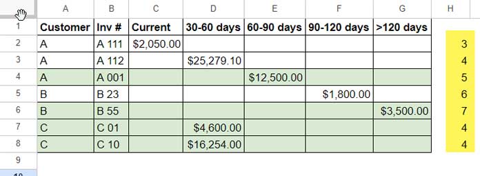
Finding the Furthest Data Point in Each Row:

BYROW(table, LAMBDA(r, XMATCH(TRUE, r<>"", 0, -1))) – Assigned the name ‘maxx’

We have employed XMATCH with BYROW to identify the last non-empty column in each row within the specified table range. BYROW plays a crucial role by iterating through each row in the range. Without it, we would be constrained to using XMATCH on a single row only.

The output of the above formula serves as a key element in identifying the records with the furthest entry in each category. The significance of this output will become apparent as you proceed through the explanations below.

Finding the last data point in each row using XLOOKUP

Sorting the Table along with the Furthest Data Point:

SORT(HSTACK(table, maxx), 1, 1, COLUMNS(table)+1, 0) – Assigned the name ‘srtA’

We utilized HSTACK to horizontally stack ‘maxx’ with ‘table’ and sorted the first column (category) in ascending order and the last column (last value positions) in descending order.

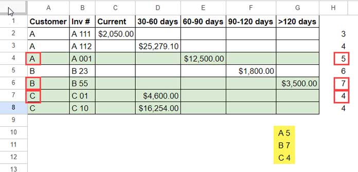
Removing Duplicates Based on Category:

SORTN(srtA, 9^9, 2, CHOOSECOLS(srtA, 1), 1) – Assigned the name ‘srtB’

The SORTN function is used to eliminate duplicates based on the category column. This will yield a table with the furthest data in each category. However, if a category has two or more rows with the same furthest data, as in the case of category C in our example, it will only return one of them.

Combining Categories and Furthest Data Points:

TRANSPOSE(QUERY(TRANSPOSE(CHOOSECOLS(srtB, {1, COLUMNS(table)+1})),,9^9)) – Assigned the name ‘combine’

TRANSPOSE -> QUERY -> TRANSPOSE (transpose the data to change orientation, query it, and transpose again) is a technique in Google Sheets to combine columns.

The purpose here is to extract the first and last columns in the SORTN result (category and furthest value position) and combine them row-wise.

Finding Rows with the Furthest Data in Each Category:

XMATCH(TRANSPOSE(QUERY(TRANSPOSE(HSTACK(CHOOSECOLS(table, 1), maxx)),, 9^9)), combine) – Assigned the name ‘fnl’

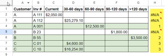
This formula identifies the rows with the furthest data entry in each category. The XMATCH function uses two arguments here: search_key and lookup_range.

The search keys consist of the category column joined with ‘maxx’, the furthest data point in each row.

The lookup range is the combined result (‘combine’).

The formula returns the relative positions in matching rows and else returns #N/A. Wherever the formula returns a number, that row represents the row with the furthest data point in each category.

Formula Expression

FILTER(table, IFNA(fnl))

This FILTER formula filters the table wherever ‘fnl’ (the result of XMATCH) returns a number.

That’s all about the formula that finds and filters the furthest data point in each category in Google Sheets.

Additional Tip: Filtering Rows with the Furthest Data in Each Category and Subcategory

If you have a category and subcategory, you should make four changes (in ‘srtA’, ‘srtB’, ‘combine’, and ‘fnl’) in the formula.

Assume the ‘table’ range is A2:F8 where A2:A8 contains categories and B2:B8 contains subcategories.

Category and subcategory-wise filtering data with the furthest data point in Google Sheets

Here are the necessary changes to be made:

SORT(HSTACK(table, maxx), 1, 1, COLUMNS(table)+1, 0) becomes SORT(HSTACK(table, maxx), 1, 1, 2, 1, COLUMNS(table)+1, 0)
SORTN(srtA, 9^9, 2, CHOOSECOLS(srtA, 1), 1) becomes SORTN(srtA, 9^9, 2, CHOOSECOLS(srtA, 1)&CHOOSECOLS(srtA, 2), 1)
TRANSPOSE(QUERY(TRANSPOSE(CHOOSECOLS(srtB, {1, COLUMNS(table)+1})),,9^9)) becomes TRANSPOSE(QUERY(TRANSPOSE(CHOOSECOLS(srtB, {1, 2, COLUMNS(table)+1})),,9^9))
XMATCH(TRANSPOSE(QUERY(TRANSPOSE(HSTACK(CHOOSECOLS(table, 1), maxx)),, 9^9)), combine) becomes XMATCH(TRANSPOSE(QUERY(TRANSPOSE(HSTACK(CHOOSECOLS(table, {1, 2}), maxx)),, 9^9)), combine)

Here is the formula after the mentioned changes:

=ArrayFormula(LET(
   table, A2:F8, 
   maxx, BYROW(table, LAMBDA(r, XMATCH(TRUE, r<>"", 0, -1))), 
   srtA, SORT(HSTACK(table, maxx), 1, 1, 2, 1, COLUMNS(table)+1, 0), 
   srtB, SORTN(srtA, 9^9, 2, CHOOSECOLS(srtA, 1)&CHOOSECOLS(srtA, 2), 1), 
   combine, TRANSPOSE(QUERY(TRANSPOSE(CHOOSECOLS(srtB, {1, 2, COLUMNS(table)+1})),,9^9)), 
   fnl, XMATCH(TRANSPOSE(QUERY(TRANSPOSE(HSTACK(CHOOSECOLS(table, {1, 2}), maxx)),, 9^9)), combine), 
   FILTER(table, IFNA(fnl))
))

This way, we can filter rows with the furthest data in each category or each category with a subcategory in Google Sheets.

Resources

We have seen two examples of filtering rows with the furthest data in Google Sheets, one with a category column and the other with a category and subcategory column.

Here are a few more tutorials that help you manage category-wise data in Google Sheets.