Filter Groups Where Any Row Meets a Condition in Google Sheets

If you’ve ever needed to filter data in Google Sheets by groups—but only keep those groups where at least one row meets a condition—this post is for you.

There are plenty of real-life situations where this is useful.

Table of Contents

Why You May Need to Filter Groups This Way

This approach comes in handy in quite a few real-world situations. Here are a couple of examples:

Inventory Management

Suppose you’re handling stock data across different stores or warehouses. You might want to list all rows related to a product, but only if it’s available somewhere — even if some rows show zero quantity. This helps you get a clearer picture of what’s currently in stock.

Project or Task Tracking

Think of a project tracker where tasks are grouped under project names. If even one task in a project is marked as “In Progress,” you may want to bring in all the tasks under that project. This way, you can focus on active projects without losing visibility into the full task list.

Let’s use the project tracking example to show how to filter groups where any row meets a condition in Google Sheets.

Sample Data

Here’s what the data might look like:

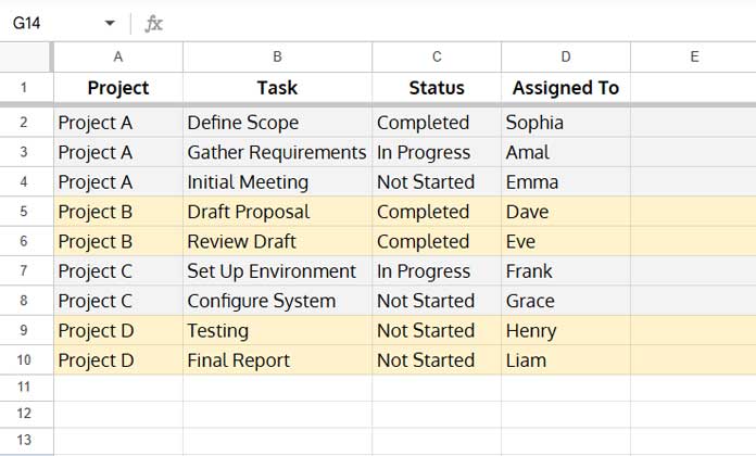
Sample project tracking data with tasks grouped by project name and status column used for filtering

In this example, Project is the group column, and we want to filter projects where any task has a status of “In Progress.”

Formula to Filter Groups Where Any Row Meets a Condition

You can use a smart combination of FILTER, UNIQUE, and XMATCH to do this.

The Formula

=FILTER(A2:D, XMATCH(A2:A, UNIQUE(FILTER(A2:A, C2:C="In Progress"))))

What the Formula Returns

This formula filters your data and keeps entire groups where at least one row in that group matches the condition—“In Progress” in this case.

Here’s what you’ll get:

Project	Task	Status	Assigned To
Project A	Define Scope	Completed	Sophia
Project A	Gather Requirements	In Progress	Amal
Project A	Initial Meeting	Not Started	Emma
Project C	Set Up Environment	In Progress	Frank
Project C	Configure System	Not Started	Grace

Only Project A and Project C are shown—because at least one task in each is marked In Progress.

Quick Breakdown of the Formula

=FILTER(A2:D, XMATCH(A2:A, UNIQUE(FILTER(A2:A, C2:C="In Progress"))))

1. FILTER(A2:A, C2:C="In Progress")
→ Pulls the project names where the status is “In Progress”

2. UNIQUE(...)
→ Keeps just one entry per matching project

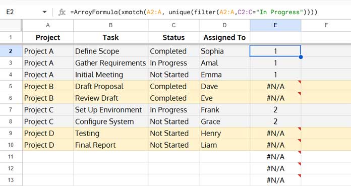
3. XMATCH(A2:A, ...)
→ Checks if each row’s project name is in that list of matching projects

Using XMATCH to filter groups where any row meets a condition in Google Sheets, returning only relevant project rows

4. FILTER(...)
→ Returns all rows where the project matched

More Use Cases

This pattern works in many other situations, like:

Showing all rows for customers who placed at least one high-value order
Returning all rows for employees with at least one late check-in
Filtering campaign data where at least one result hit a conversion goal