In Google Sheets, when you want to use XLOOKUP to find a value in a column and retrieve a value from the row above or below, you can utilize OFFSET with it.

Similarly, in horizontal lookup, you can employ OFFSET with XLOOKUP in Google Sheets. This allows you to search for a value in a row and return a value from the column to its left or right.

XLOOKUP with OFFSET to Return a Value from the Row Below or Above

Below, you will find three examples:

1. Exact Match and Search from First Value to Last Value + Offset.
2. Exact Match and Search from Last Value to First Value + Offset.
3. Wildcard Match + Offset.

Here are the syntaxes of the XLOOKUP and OFFSET functions for your quick reference:

XLOOKUP: XLOOKUP(search_key, lookup_range, result_range, [missing_value], [match_mode], [search_mode])

• search_key: The value to search for.
• lookup_range: The range to search within.
• result_range: The range to retrieve values from.
• missing_value: (Optional) The value to display if no match is found.
• match_mode: (Optional) 0 (exact match), 1 (exact match or next larger), -1 (exact match or next smaller), 2 (wildcard match).
• search_mode: (Optional) 1 (search first to last), -1 (search last to first), 2 (binary search in ascending sorted range), -2 (binary search in descending sorted range).

Ref.: How to Use the XLOOKUP Function in Google Sheets

OFFSET: OFFSET(cell_reference, offset_rows, offset_columns, [height], [width])

• cell_reference: The starting cell reference.
• offset_rows: The number of rows to offset (positive or negative).
• offset_columns: The number of columns to offset (positive or negative).
• height: (Optional) The height of the range to be returned.
• width: (Optional) The width of the range to be returned.

Ref.: OFFSET Function in Google Sheets and Dynamic Ranges – Examples

Example 1: Retrieve the Value from the Row Below

In this example, we need to find the salary of Lisa, which is presented below the row that contains her name.

=OFFSET(XLOOKUP(D1, A1:A, B1:B), 1, 0)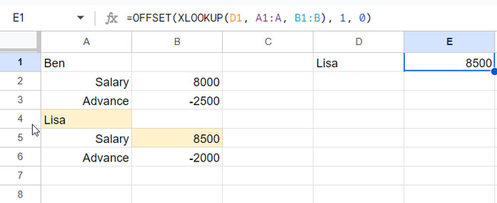

The criterion (search_key) is in cell D1 in the above formula.

The XLOOKUP searches this key in A1:A (lookup_range) and returns the corresponding value from B1:B (result_range). Since we want the XLOOKUP to return the value in the row below, we have employed the OFFSET.

The OFFSET function offsets 1 row (offset_rows) and 0 columns (offset_columns) from the XLOOKUP result cell (cell_reference).

In this formula, you can specify the height and width arguments if desired. For example, if you want to retrieve the salary and advance of Lisa, which are in the rows below her name, you can use the formula as follows:

=OFFSET(XLOOKUP(D1, A1:A, B1:B), 1, 0, 2)

Example 2: Retrieve the Value from the Row Above

Consider a list of items in column A, such as fruit names. You want to find the item’s name immediately above the last occurrence of a specific item (e.g., “apple”).

=OFFSET(XLOOKUP(C2, A2:A, A2:A, , 0, -1), -1, 0)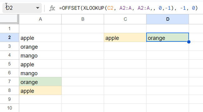

In this formula, C2 contains the search_key “apple”. The XLOOKUP searches for the key from the last value to the first value (search_mode -1) in the lookup_range and returns the value itself. The OFFSET function offsets -1 row (offset_rows) and 0 columns (offset_columns).

This means the XLOOKUP and OFFSET combo returns the value from the row above the XLOOKUP result value.

Example 3: Using XLOOKUP with OFFSET and Wildcard Match

Suppose we have a table with Product Names, Categories, and Prices in columns A, B, and C, respectively.

We want to perform a wildcard match for “Lamp” in product names and return its price. The twist here is that we don’t want the price of the lookup item, but the price of the item below it.

This is because we need to find what amount we spent immediately after the lamp’s purchase.

=OFFSET(XLOOKUP("*Lamp*", A1:A, C1:C, ,2), 1, 0)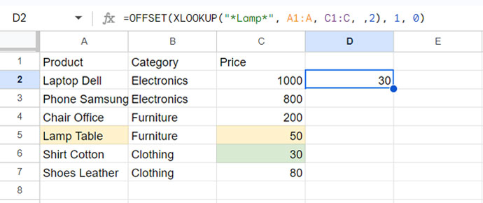

The above formula uses wildcard matching (match_mode 2) in XLOOKUP and offsets 1 row to fetch the value from the row below.

In all examples, you can offset more than 1 row, either down (positive) or up (negative).

XLOOKUP with OFFSET to Return a Value from the Column to the Left or Right

You may well be aware that XLOOKUP is capable of performing horizontal lookup as well.

In all the above three examples, we have used XLOOKUP with OFFSET for vertical lookup and offsetting rows up or down.

If your lookup_range is a row and the result_range is the same row or another row, then you need to OFFSET columns, not rows, to get the value to the left or right of the result column.

I’ll share one example below. In this example, XLOOKUP will search for a key in a row and offset one column to the right. You can follow that example to offset columns to the left and also apply the last value to the first value search, the first value to the last value search, or the wildcard match.

Suppose a person is assigned three tests. The sample data in the row contains his first test date, result, second test date, result, third test date, and result.

We need to find his most recent test result. So we will search for today’s date and offset 1 column to get the result from the next column of the XLOOKUP result column.

=OFFSET(XLOOKUP(TODAY(), C2:H2, C2:H2, ,-1), 0, 1)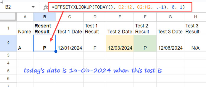

The formula searches for the criterion TODAY() (search_key) in C2:H2 and returns the date that is less than or equal to the search key (match_mode -1) in the same range. The OFFSET offsets 0 rows (offset_rows) and 1 column (offset_columns) to return the result of that most recent test.

This is another example of XLOOKUP and offset results in Google Sheets.

Resources

More XLOOKUP formula examples for enthusiasts.

1. XLOOKUP Visible (Filtered) Data in Google Sheets
2. XLOOKUP Nth Match Value in Google Sheets
3. Nested XLOOKUP Function in Google Sheets
4. VLOOKUP and XLOOKUP: Key Differences in Google Sheets
5. XLOOKUP with Multiple Criteria in Google Sheets
6. XLOOKUP for Multiple Column Results in Google Sheets
7. XLOOKUP with Date and Time in Google Sheets
8. XLOOKUP with Single IMPORTRANGE & LET in Google Sheets