INDEX-MATCH: Better Alternative to VLOOKUP and HLOOKUP

INDEX-MATCH is a better alternative to VLOOKUP and HLOOKUP in Google Sheets. It is not a single function, but rather a combination of two Google Sheets lookup functions: INDEX and MATCH.

You can use the INDEX and MATCH functions together to create a more robust and flexible lookup function than VLOOKUP or HLOOKUP.

Before we discuss the benefits of using INDEX-MATCH over VLOOKUP and HLOOKUP, let’s see how to use each function independently.

You will learn about the INDEX, MATCH, VLOOKUP, and HLOOKUP functions in this article. However, I have detailed tutorials on each one of them.

Must Check: Google Sheets Function Guide.

INDEX Formula

Syntax of the INDEX Function:

INDEX(reference, [row], [column])

The primary purpose of Google Sheets Lookup formulas is to return the content of a cell based on a search key or offset number.

In the INDEX formula, we can use offset row numbers and column numbers to return the specific content of a cell.

Here is an example:

=INDEX(A2:G7,5,3)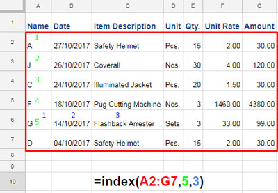

A2:G7 is the lookup range (reference),
5 is the row offset, and
3 is the column offset.

This formula would return “Flashback Arrester” as the result.

Study the above example carefully. Once you have learned it, we can move on to the example of the MATCH function, the second function in the INDEX-MATCH combo in Google Sheets.

MATCH Formula

Syntax of the MATCH Function:

MATCH(search_key, range, [search_type])

The MATCH is another lookup formula in Google Sheets that can be used independently or in combination with the INDEX function.

The MATCH formula can be used for vertical or horizontal lookups. However, the MATCH formula returns the relative position of the search key, not the value itself. To get the value, we need to use the combination of INDEX and MATCH in Google Sheets.

In the Google Sheets MATCH function, the range must be a one-dimensional array, either horizontal or vertical.

1. Vertical Use of MATCH Formula in Google Sheets

In the following formula, the search key is “Flashback Arrester”, the lookup range is C2:C7, and the match type is 0, which indicates that the data is not sorted.

=MATCH("Flashback Arrester",C2:C7,0)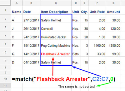

The MATCH formula would return the number 5, which is the relative position of the item, i.e., “Flashback Arrester”, in the range or array.

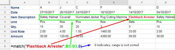
2. Horizontal Use of MATCH Formula in Google Sheets

When you have a horizontal data set, you should use the MATCH formula horizontally. Here is an example:

=MATCH("Flashback Arrester",B3:G3,0)

It is similar to the vertical use of the MATCH formula. So I will not go into the details.

Learn the above two functions thoroughly. Then move on to the below examples of INDEX-MATCH combined use in Google Sheets.

How to Use INDEX-MATCH in Google Sheets

In the following example, we will use the Figure 1 and 2 examples. That is, we will use the INDEX and MATCH formulas in a vertical dataset.

We have used the following formula to offset 5 rows in the third column in the range A2:G7 to return the item “Flashback Arrester”.

=INDEX(A2:G7,5,3)

If you do not know which row the said item is in, you can use the following MATCH to get the relative position.

=MATCH("Flashback Arrester",C2:C7,0)

That means we can replace the row offset, that is, 5 in the above INDEX formula with the above MATCH formula.

Here is that INDEX-MATCH formula in Google Sheets.

=INDEX(A2:G7,MATCH("Flashback Arrester",C2:C7,0),3)

We usually do not want to return the search item as above. We may need a value from the same row from another column. The below INDEX-MATCH combo matches “Flashback Arrester” in the third column and returns a value from the seventh column.

=INDEX(A2:G7,MATCH("Flashback Arrester",C2:C7,0),7)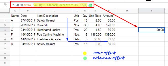

INDEX-MATCH with Multiple MATCH Functions

Here is the most exciting part. In the above INDEX-MATCH formula, I have used the MATCH formula to replace the row offset of 5. However, the column offset of 7 is hard-coded.

This is because we know that the 7th column contains the “Amount”. However, if you want, you can use MATCH to find the relative position of “Amount” in the header row and use that as the column offset in INDEX.

This is the MATCH formula:

=MATCH("Amount",A1:G1,0)

And here is the updated INDEX-MATCH formula with multiple MATCH functions.

=INDEX(A2:G7,MATCH("Flashback Arrester",C2:C7,0),MATCH("Amount",A1:G1,0))

We are talking about how INDEX-MATCH is a better alternative to VLOOKUP and HLOOKUP in Google Sheets. So let’s move on to how to use the V/H LOOKUP formulas in Google Sheets.

VLOOKUP Formula

VLOOKUP Syntax in Google Sheets:

VLOOKUP(search_key, range, index, [is_sorted])

Note: The index is an argument within the VLOOKUP formula, not the INDEX function. It’s for specifying the return value (result) column.

The VLOOKUP formula searches down the first column of the range for a given search key. It then returns the value in the same row from the specified column.

So, when we replace the INDEX-MATCH formula with the VLOOKUP, we must use the range C2:G7 instead of A2:G7 because the search key is present in C2:C7.

So the “Amount” column number is 5, not 7. Here is the alternative to the above INDEX-MATCH formula:

=VLOOKUP("Flashback Arrester",C2:G7,5,0)

Where:

"Flashback Arrester" is the given search key.
C2:G7 is the range.
5 is the column index.
0 specifies that the data is not sorted.

HLOOKUP Formula

HLOOKUP Syntax in Google Sheets:

HLOOKUP(search_key, range, index, [is_sorted])

You can use the HLOOKUP formula for horizontal lookups. In the following example, the HLOOKUP formula matches “G” in B1:G1 in the range B1:G7, and returns the value from the found column in row # 3.

=HLOOKUP("G",B1:G7,3,0)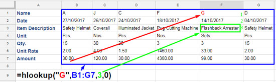

Horizontal lookup formula example — Figure 5

INDEX-MATCH Formula: A Better Alternative to VLOOKUP and HLOOKUP

In the following examples, we will see the VLOOKUP and HLOOKUP formulas and their alternative INDEX-MATCH formulas.

The following VLOOKUP formula searches down the key “G” in A2:G12 and returns the value from the third column of the matching row.

=VLOOKUP("G",A2:G7,3,0)

Here is the VLOOKUP alternative INDEX-MATCH formula:

=INDEX(A2:G7,MATCH("G",A2:A7,0),3)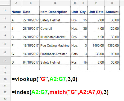

INDEX-MATCH Example 2 (VLOOKUP) — Figure 6

In the same way, you can use the INDEX-MATCH formula for horizontal lookups. Please see the two formulas below.

HLOOKUP:

=HLOOKUP("G", B1:G7, 3, 0)

INDEX-MATCH Alternative:

=INDEX(B1:G7, 3, MATCH("G", B1:G1, 0))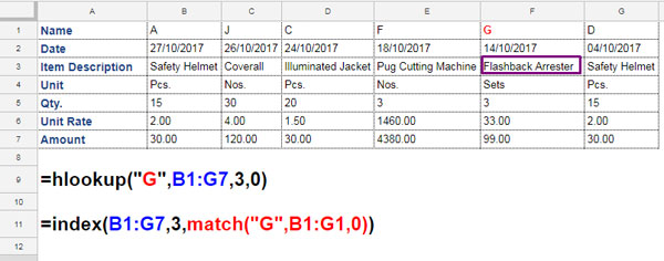

INDEX-MATCH Example 3 (HLOOKUP) — Figure 7

Advantages of Using INDEX-MATCH Over VLOOKUP and HLOOKUP in Google Sheets

This is the pros and cons part, and I will only touch the core part.

First, we will start by answering the question: Why should you switch to INDEX-MATCH from VLOOKUP or HLOOKUP formulas?

Pros

Most Google Sheets and Excel users are aware of the use of the VLOOKUP function. I think this is because of the word-of-mouth publicity it gets among spreadsheet users. So I think the importance of the INDEX-MATCH combination is somewhat undermined.

Now to the point. Instead of telling you what VLOOKUP can do, I will tell you what VLOOKUP can’t do (without workarounds).

Here are some of the advantages of INDEX-MATCH over VLOOKUP and HLOOKUP:

1. Left Side Lookups

The VLOOKUP formula looks up the first column of a range, so it cannot return a value left of the search key.

See the below example.

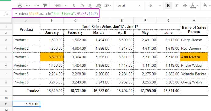
In the example below, the search key is “Ann Rivera”, which is in the last column of the range. There is no option in regular VLOOKUP to return a value left to the lookup value. I have done it with the INDEX-MATCH formula below.

=INDEX(A3:H8,MATCH("Ann Rivera",H3:H8,0),2)

Here we want to know the sales value of Ann Rivera in January. With the INDEX-MATCH combo, I have addressed this issue.

INDEX-MATCH Example 4 (Left Side Lookup) — Figure 8

I was talking about the incapability of the regular VLOOKUP formula to return a value left of the search key. However, there is a workaround that we can use to address this issue.

=VLOOKUP("Ann Rivera",HSTACK(H3:H8,A3:G8),3,0)

Now, Google Sheets has a new lookup function called XLOOKUP that can be used for left-side lookups.

=XLOOKUP("Ann Rivera",H3:H8,B3:B8)

2. New Column Issue in Lookup

The VLOOKUP formula below searches down the key “Product 4” in column A and returns the value from the same row (the search key found row) from column 4, i.e., 1396.00.

=VLOOKUP("Product 4",A3:H8,4,0)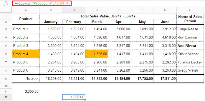

The problem here is that if you insert a new column between column 1 and column 4, you will get a wrong answer. For example, if the new column is just left to column 4 and it’s blank, you will get blank.

Again, the INDEX-MATCH formula combo can solve this issue. See the alternative INDEX-MATCH formula below.

=INDEX(E3:E8,MATCH("Product 4",A3:A8,1),1)

Here is the workaround XLOOKUP.

=XLOOKUP("Product 4",A3:A8,E3:E8)

All of the above drawbacks of VLOOKUP are also applicable to HLOOKUP.

Cons

One of the main disadvantages of the INDEX-MATCH formula over VLOOKUP or HLOOKUP is that it cannot return an array result. However, advanced users can solve this limitation with lambda functions such as BYROW, BYCOL, or MAP with INDEX-MATCH.

Resources

16 COMMENTS

Jaziel December 2, 2020 At 1:54 am

This was a magical fix to what I struggled to do all day. Quick fix. THANKS!!!!

Dani Goffi May 29, 2020 At 11:56 am

Hello,

Thanks for sharing this with us. I am having trouble figuring out how to get google sheets to do what I need it to and I hope you are up for a challenge 😀

Here is a sample sheet: — link removed by admin —

When I export my orders into sheets, each product people purchase appears on a new line. These are in no particular set order, as they depend on how the person has added items into their cart.

Some people have one product (and one line), some have multiple products/lines, and there is some extra lines/info like shipping, delivery, and discount codes that are irrelevant.

Products also have variances (like Large or Small) but that data is contained within the product_title column

I want to be able to get the sheet to bring back what size of the box they have. If they have fruit, and if they have any add on (broccoli used for this example)

At the moment I am using filters and helper sheets plus a combination of vlookups+IF+IFERROR to accomplish the task, but I am sure there must be a better way!

Thanks for your help.

- Prashanth May 30, 2020 At 4:25 pm
  
  Hi, Dani Goffi,
  
  I could try if you share the editable version of your sheet. Also in that sheet, please explain more details like show me your result, and logic.
  
  Best,
  
Eddy A September 29, 2019 At 8:14 pm

Sorry I meant:

I need to check if the codes were scanned for the correct department (column C on my current sheet)

So when I copy the formulas down they look like this:

=INDEX('S2'!$A:$AJ, MATCH($C3, 'S2'!D:D, 0), MATCH("Department", 'S2'!$1:$1, 0))

then C4, C5,…

Guess it’s time to get some sleep.

- Prashanth September 30, 2019 At 9:27 am
  
  Hi, Eddy,
  
  I have tried to replicate a sample data as per your explanation but failed miserably.
  
  If you can prepare a sample sheet which contains your ‘current sheet’ (formula tab), tab ‘S2’ and one more tab with your expected result, I would be able to help you.
  
  You can’t use Index-Match to expand the result as required. The better solution may be Vlookup, that I can only check once you Share your example Sheet.
  
  Best,
  
  - Eddy A September 30, 2019 At 10:28 am
    
    Dear Prashanth,
    
    I’ve created an example sheet with my private account and made it public:
    
    S1: inventory data from our ERP system.
    
    S2: data from the agents that scan assets for each department.
    
    Calculations column A: checks if an asset was scanned or not.
    
    Calculations columns B:J: Shows the S1 data (formula in column A compares to C).
    
    Calculations columns K:Q: My formulas to check the department based on the scanned asset code. This is where I need help.
    
    Calculations column R: Next I want to compare the department from the column I with K:Q and show the FALSE entries to our inventory coordinator so he can fix it. So maybe you can combine this with 1 VLOOKUP formula with an array that replaces columns K:R and would just show TRUE, FALSE or BLANK?
    
    I’ve filled R out manually to show what I mean.
    
    Thank you for your willingness to help me with this.
    
    Best, Eddy
    
    - Prashanth September 30, 2019 At 2:51 pm
      
      Hi, Eddy,
      
      Added the formulas in K2:R2.
      
      The following formula in K2 dragged to the right until Q2.
      
      =ArrayFormula(IFNA(VLOOKUP($C$2:$C,{'S2'!C2:C,'S2'!$B$2:$B},2,0)))
      
      Then here is the formula used in R2.
      
      =ArrayFormula(if(len(I2:I),IF((I2:I=K2:K)+(I2:I=L2:L)+(I2:I=M2:M)+(I2:I=N2:N)+(I2:I=O2:O)+(I2:I=P2:P)+(I2:I=Q2:Q)>0,TRUE,FALSE),))
      
      Hope this helps?
      
      Best,
      
      - Eddy A September 30, 2019 At 3:51 pm
        
        I had to drag a little further and extend your second formula a little for the 30 columns in my original sheet but it works perfectly. I’m extremely grateful for your swift and professional assistance.
        
        Respect to you and have a lovely day!
        
        Eddy
Eddy A September 29, 2019 At 8:09 pm

I’m trying to get my formula to work better:

=INDEX('S2'!A:AJ, MATCH(C2, 'S2'!C:C, 0), MATCH("Department", 'S2'!1:1, 0))

On sheet S2 I have 30 columns with QR codes since we scan 30 at a time. Column C in sheet S2 has the department names from each scan session.

I need to check if the codes were scanned for the correct department (column C:C on my current sheet) by comparing the department from each row where a QR code is found but the QR code can be in any of the 30 columns (D:AJ) in S2.

I’ve been working on this all weekend. Your article is the best I can found but I can’t get it to work in an array so my only solution is to add $ and drag it right 30 times:

Formula # 1

=INDEX('S2'!$A:$AJ, MATCH($C2, 'S2'!D:D, 0), MATCH("Department", 'S2'!$1:$1, 0))

Formula # 2

=INDEX('S2'!$A:$AJ, MATCH($C2, 'S2'!E:E, 0), MATCH("Department", 'S2'!$1:$1, 0))

… and then drag those 30 formulas down (+2,000 rows in the real database so +60,000 formulas making it slow to update and probably will hit Google quotas).

I can’t share the sheet outside of our company network but I hope there’s a better way? Please help?

Pablo alvarez August 13, 2019 At 4:14 pm

Is possible to use Arrayformula with Index?

For example.: range = A:E, [rows] = N:N

=ARRAYFORMULA(index(A:E;N:N;5))

- Prashanth August 14, 2019 At 9:01 am
  
  Hi, Pablo alvarez,
  
  The Index itself is an Array Function. So it won’t take or require to use ArrayFormula with it.
  
  Can you please explain what you are trying to do with that formula?
  
Sven Van Dyck June 6, 2019 At 3:04 pm

Hi, I was wondering/struggling.

I have a list with:

– Column A: contains values (numbers)
– Column B: references (in this case unique values (aka countries))

Now the idea is that I have made a ranking of the figures in Column A (1-10) for reporting reasons using LARGE and I want to display the reference next to that ranking. I need that reference for additional reporting…

Here is the problem: If I rank a top 10 I will get eg. 3 times the same value, a VLOOKUP or INDEX/MATCH, however, will always return the same value as a reference.

Question: How do I get a formula to move on to the next value so the references are different

- Prashanth June 6, 2019 At 5:52 pm
  
  Hi, Sven Van Dyck,
  
  Please share an example Sheet in Edit or View mode. Please do include the result that you are expecting.
  
  Let me copy the data and try.
  
  Thanks.
  
  - Sven Van Dyck June 6, 2019 At 7:41 pm
    
    Hi Prashanth,
    
    Thank you for replying so fast!
    
    It is an enormous file, so I reduced it to the required sheet. I highlighted the problem. We have the same values based upon the original numbers… I included the expected outcome in a separate column…
    
    Note: Sheet’s link removed by the admin.
    
    Thanks a million if you can make this work.
    
    - Prashanth June 7, 2019 At 4:46 pm
      
      Hi, Sven Van Dyck,
      
      Please forget about the Vlookup and Index-Match. Use the below Query. You can easily adapt to it and modify.
      
      Formula 1 (Belgium Top Traffic Lanes – Outbound)
      
      Note: The below formula will expand to rows and columns. So make enough room (10 rows x 3 columns). Better try it in a new tab.
      
      =Query(Trial_1!$E$3:$J,"Select E,J,I order by E Desc limit 10")
      
      Formula 2 (Formula 1 (Belgium Top Traffic Lanes – Inbound)
      
      =Query(Trial_1!$E$3:$J,"Select F,J,I order by F Desc limit 10")
      
      Now see the formulas. I have used the same data ranges in both the formulas. Only changed the outbound/inbound columns.
      
      The idea is sorting the inbound/outbound columns in descending order and limiting the output to 10. I hope now you can code this formula for the other country.
      
      Hope you got the point.
      
      Update:
      
      Italy: Outbound
      
      =Query(Trial_1!$E$3:$J,"Select G,J,I order by G Desc limit 10")
      
      Italy: Inbound
      
      =Query(Trial_1!$E$3:$J,"Select H,J,I order by H Desc limit 10")
      
      Best,
      
      - Sven Van Dyck June 7, 2019 At 7:11 pm
        
        You have me completely stunned. Thank you so much!