The SEQUENCE function combined with date functions allows you to generate a sequence of months or month endings in Google Sheets.
Although you can replace the SEQUENCE function with the ROW function, I recommend sticking with the former due to its flexibility.
Here are the advantages of using SEQUENCE over ROW in this context:
- Orientation Flexibility: You can easily switch the orientation of the result from rows to columns or vice versa without needing to use TRANSPOSE.
- Descending Order: SEQUENCE allows you to generate a sequence of months in descending (reverse chronological) order without needing to use SORT.
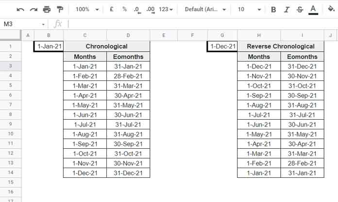
In this post, there are four formulas included, all of which output values vertically. You can refer to the four columns in the image below for visualization.
I’ll further explain how to switch the orientation and provide more details under the relevant sections below.
Generating Chronological Sequence of Months or End-of-Months in Google Sheets
Result in a Column (Vertically)
Let’s say you want to create a sequence of months for the year 2021.
In cell B1, input the date 2021-01-01, then enter the following formula in cell C3 (refer to the image above):
=ArrayFormula(EDATE(B1,SEQUENCE(12, 1, 0)))This formula generates the sequence of the beginning-of-month dates vertically in the range C3:C14.
To obtain the sequence of end-of-month dates, use the following formula in cell D3 (see the range D3:D14 in the screenshot above):
=ArrayFormula(EOMONTH(EDATE(B1,SEQUENCE(12, 1, 0)), 0))Both formulas take the input, i.e., start date, in cell B1 and generate the result.
Formula Explanation
Let’s break down the first formula. The second formula requires a minor adjustment.
First, input the following EDATE formula in any blank cell. But before that, enter the date 2021-01-01 in cell B1.
=EDATE(B1, 0)This will return the date 1-Jan-21. Now, modify the formula as follows:
=EDATE(B1, 1)This will return the date 1-Feb-2021.
The syntax of the EDATE function is EDATE(start_date, [months])
From the above two formulas, you can deduce one thing: when you use the SEQUENCE function in the ‘months’ argument, generating a sequence from 0 to 11, you will get a sequence of months.
The following formula accomplishes this:
SEQUENCE(12, 1, 0)Syntax: SEQUENCE(rows, [columns], [start], [step])
So, the EDATE function will generate a sequence of 12 months in chronological order.
To obtain the end-of-month sequence, we utilized the EOMONTH function to convert the beginning of the month to the end of the month.
Syntax: EOMONTH(start_date, months)
Where:
start_date: represents the beginning of the month date.months: set to 0 (indicating the last day of the provided start date).
Result in a Row (Horizontally)
Earlier, we highlighted the flexibility of the SEQUENCE function. Now, let’s put it to the test.
To generate a sequence of months or end-of-months horizontally in Google Sheets, follow these steps:
Start with our existing SEQUENCE formula:
SEQUENCE(12, 1, 0)In both the C3 and D3 formulas, modify it as follows:
SEQUENCE(1, 12, 0)This adjustment will produce the sequence of months horizontally.
Note: You should move the D3 formula to C4; otherwise, it will prevent the C3 formula from expanding, resulting in a #REF error.
Sequence of Months or End-of-Months in Reverse Order in Google Sheets
To obtain the sequence of months in reverse order vertically, start by entering the first date of December as the start date. For example, for 2021, follow these steps:
Enter the date 2021-12-1 in cell G1 and insert the following formula in cell H3 (refer to our earlier screenshot above):
=ArrayFormula(EDATE(G1, SEQUENCE(12, 1, 0, -1)))This will return the beginning-of-month dates in reverse chronological order.
Next, use the following formula in cell I3 to get the sequence of end-of-months in reverse chronological order:
=ArrayFormula(EOMONTH(EDATE(G1, SEQUENCE(12, 1, 0, -1)), 0))The difference in these two formulas compared to our earlier ones is the step value -1 in the SEQUENCE function, resulting in a sequence from 0 to -11.
To display the output across the row, replace SEQUENCE(12, 1, 0, -1) with SEQUENCE(1, 12, 0, -1).


