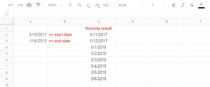
If you have a start date in cell A2 and an end date in cell B2, you might wonder how to increment the months between these two dates. This is a common requirement for many spreadsheet users.

To achieve this, we can utilize a combination of the DATEDIF, SEQUENCE, EDATE, and ARRAYFORMULA functions.

Example Setup

In the following example, the start date is in cell A2 (05/10/2017), and the end date is in cell B2 (11/06/2018). The resulting month sequence would be:

05/10/2017
05/11/2017
05/12/2017
05/01/2018
05/02/2018
05/03/2018
05/04/2018
05/05/2018
05/06/2018

If you prefer to list the start dates of each month, you can enter 01/10/2017 and 01/06/2018 in cells A2 and B2, respectively.

Formula to Increment Months Between Two Given Dates

Formula:

=ARRAYFORMULA(
   EDATE(
      A2, 
      SEQUENCE(DATEDIF(A2, B2, "M") + 1, 1, 0)
   )
)

Explanation of the Formula

• DATEDIF(A2, B2, "M"): This function calculates the number of complete months between the two dates in A2 and B2.
• SEQUENCE(…): This function generates a sequence of numbers from 0 to n, where n is the value returned by the DATEDIF function. The addition of + 1 ensures that the last month is included in the output.
• EDATE(A2, …): This function returns a date that is a specified number of months before or after the start date (A2). Here, it uses the sequence of numbers generated to increment the months accordingly.

Since the months argument (with the syntax EDATE(start_date, [months])) in the EDATE function consists of multiple values (the sequence), we must use ARRAYFORMULA to output the entire sequence of dates.

Additional Tips

To generate the start dates of each month, you can enter the first day of the month (e.g., 01/10/2017 for October) in cell A2 and the first day of the last month (e.g., 01/06/2018 for June) in cell B2. However, this is not the only way to achieve the same result.

To populate the month-end dates instead, use the following formula:

=ARRAYFORMULA(
   EOMONTH(
      EDATE(
         A2, 
         SEQUENCE(DATEDIF(A2, B2, "M") + 1, 1, 0)
      ), 0
   )
)

If you wish to calculate the start date of each month, use this formula:

=ARRAYFORMULA(
   EOMONTH(
      EDATE(
         A2, 
         SEQUENCE(DATEDIF(A2, B2, "M") + 1, 1, 0)
      ), -1
   )+1
)

Resources for Further Reading

• Generating a Sequence of Months in Google Sheets
• Expand Dates and Assign Values in Google Sheets (Array Formula)
• How to Auto-Populate Dates Between Two Given Dates in Google Sheets
• Populate an Entire Month’s Dates Based on a Drop-down in Google Sheets
• How to Populate Sequential Dates Excluding Weekends in Google Sheets
• How to Increment DateTime by One Hour in Google Sheets (Array Formula)
• Incrementing Duplicate Dates by Month or Day in Google Sheets
• Date Sequence Every Nth Row in Excel (Dynamic Array)