Finding the median for grouped data in Google Sheets can be tricky because the QUERY function doesn’t include a median calculation. Fortunately, pivot tables in Google Sheets provide a simple solution.
In this tutorial, you’ll learn:
- How to calculate item-wise median using formulas
- How to calculate item-wise median using a pivot table
- Why pivot tables are often the easier, more scalable solution
This article is part of the Pivot Table Calculations & Advanced Metrics in Google Sheets hub.
Step 1: Sample Dataset
Here’s the dataset we’ll use for this example:
| Project | Bid Price |
|---|---|
| Project 1 | 5000 |
| Project 1 | 5500 |
| Project 1 | 6500 |
| Project 1 | 6600 |
| Project 1 | 7000 |
| Project 2 | 12000 |
| Project 2 | 14300 |
| Project 2 | 15000 |
| Project 2 | 18000 |
We want to find the median bid for each project.
Step 2: Using Formulas for Item-wise Median
You can calculate median per project without a pivot table using MEDIAN + FILTER or MEDIAN + IF formulas.
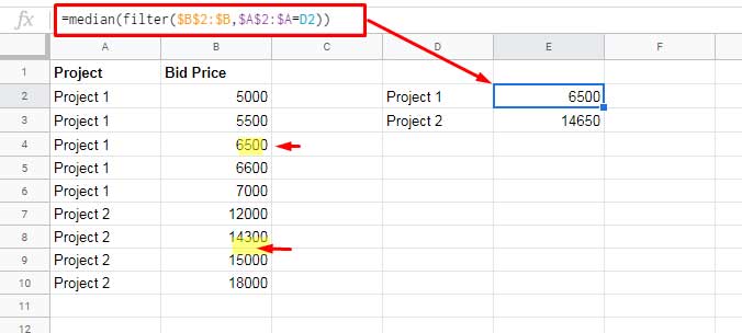
Option 1: MEDIAN + FILTER
- Enter unique project names in
D2:
=UNIQUE(A2:A)
- Calculate median for each project in
E2:
=MEDIAN(FILTER($B$2:$B, $A$2:$A=D2))
- Copy the formula down for all projects.
Option 2: MEDIAN + IF (Array Formula)
=ArrayFormula(MEDIAN(IF($A$2:$A=D2, $B$2:$B)))
- Returns the same result
⚠️ Tip: These formulas work well for small datasets but can get complex for large datasets. Pivot tables are simpler and more scalable.
Step 3: Using a Pivot Table for Item-wise Median
Pivot tables are usually the easier and faster way to calculate item-wise medians.
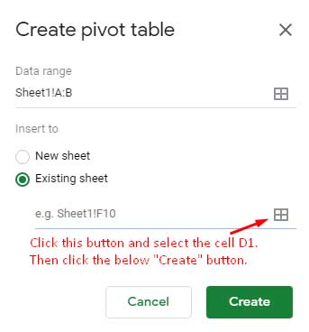
Step 3a: Create Pivot Table
- Select your data range (
A:B) - Go to Insert > Pivot Table
- Choose to place the pivot table in the same sheet or a new sheet
Step 3b: Configure Pivot Table
- Add Project under Rows
- Add Bid Price under Values
- Change Summarize by to Median
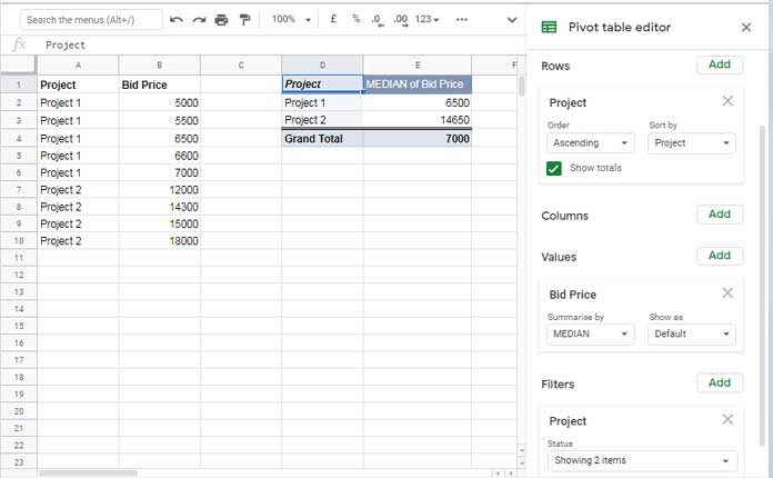
⚠️ Note: The Grand Total row does not calculate a meaningful median and can be hidden if desired.
Step 3c: Filter (Optional)
If your source data contains blank rows in the Project column, the pivot table may return #NUM! errors. To prevent this:
- In the Pivot Table Editor, go to Filters → Add → Project.
- Choose Filter by condition → Custom formula is.
- Enter the following formula:
=NOT(ISBLANK(A2:A))
- Click OK.
Your pivot table will now exclude blank rows and display the correct item-wise median for each project.
Step 4: Comparison & Recommendation
- Formulas: Flexible, good for advanced scenarios, but harder to maintain on large datasets
- Pivot Table: Easier to use, automatically updates with new data, and scales well
For most use cases, I recommend pivot tables for calculating item-wise median in Google Sheets.
Sample Sheet
A sample Google Sheets file is included at the end of this tutorial so you can explore the pivot table and formulas in action.
Conclusion
Calculating item-wise median in Google Sheets is straightforward once you know your options.
- For small datasets or quick calculations, formulas like
MEDIAN + FILTERorMEDIAN + IFwork well. - For larger datasets, or when you want automatic updates and easier reporting, pivot tables are the most efficient solution.
By following this tutorial, you can now:
- Quickly find median values per item or project
- Compare formula-based and pivot table approaches
- Apply the same techniques to any grouped data in your Google Sheets
Don’t forget to check the sample Google Sheets file at the end of this post to practice and verify your results.
Once you’re comfortable with median calculations, explore other advanced pivot table metrics in our Pivot Table Calculations & Advanced Metrics hub to supercharge your reporting in Google Sheets.


