If you understand what the median is and how to calculate it manually, using the MEDIAN function in Google Sheets becomes straightforward.
In this tutorial, you’ll learn three things: what the median is, how to calculate it manually, and how to utilize the MEDIAN function in Google Sheets.
Once you’ve mastered using the MEDIAN function, you can explore conditional (MEDIAN IF) and group-wise median in Google Sheets. Additionally, learn how to handle hidden or filtered rows in median calculations.
Median – How to Manually Calculate it
The median is the central value within a dataset. However, before determining the median, it’s essential to arrange the values in ascending order (in spreadsheet terms, you can think of it as sorting from A to Z). Then, you can identify the middle value.
Example:
For the numbers 1, 6, and 5, the median is 5. How? By arranging the values in ascending order: 1, 5, and 6. The middle number, 5, is then identified as the median.
Two crucial points are involved in calculating the median. Understanding these points is essential for effectively utilizing the MEDIAN function in Google Sheets. What are they?
1. Odd Number of Values
In the example provided, there are a total of five numbers, constituting an odd count of values. Here’s an example of median calculation with an odd number of values:
Find the median of the numbers 1, 3, 6, 10, and 9. Since there are five numbers, it’s also an odd count.
In this case, the median, or middle number, is 6. However, the calculation differs when dealing with an even count of values in the median.
2. Even Number of Values
Find the median of the following set of even values: 3, 5, 9, and 10. There are four numbers, indicating an even count.
With four numbers, it’s not possible to select a single middle value. Instead, choose two middle values and determine their average. This average represents the median.
In the provided set of numbers, 5 and 9 are the middle values. Adding them yields a total of 14. Therefore, the average is 14 divided by 2, resulting in 7. Hence, 7 is the median of the given numbers.
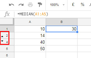
How to Use the MEDIAN Function in Google Sheets
When utilizing the MEDIAN function, there’s no need to worry about sorting the values or whether they are odd or even. Moreover, in a large dataset, manually calculating the median can be challenging.
Syntax:
=MEDIAN(value1, [value2, …])Arguments:
value1– The first value or range to consider when calculating the median.value2, … – Additional values or ranges. This argument is optional and useful when inputting values directly.
Examples:
=MEDIAN(5, 4, 1) // returns 4In the above formula, we’ve specified value1, value2, and value3. In the following formula, we’ve specified the range A1:A6.
=MEDIAN(A1:A6)
MEDIAN IF (Conditional Median)
There isn’t a specific MEDIANIF() function in Google Sheets. However, to evaluate values before finding the middle value, you can combine the IF function with the MEDIAN function.
For instance, let’s exclude 0 values and determine the middle value using the MEDIAN and IF combination in Google Sheets.
Suppose the values in A1:A5 are 0, 10, 20, 30, and 40. The middle value is 20. Excluding 0, the middle value becomes 25.
Here’s the MEDIAN IF formula:
=ArrayFormula(MEDIAN(IF(A1:A5>0, A1:A5)))The IF function checks if the values in the range A1:A5 are greater than 0. If TRUE, it returns the value; otherwise, it returns FALSE.
The MEDIAN function excludes FALSE while calculating the middle value.
The ArrayFormula function is necessary since we’re using IF over a range, not a single cell.
Here’s another example of using MEDIAN IF in Google Sheets:
Let’s say you have sales figures for January to March in A2:C5, where A2:A5 contains January sales, B2:B5 contains February sales, and C2:C5 contains March sales.
You can apply MEDIAN IF as follows:
=ArrayFormula(MEDIAN(IF(A2:C5>0, A2:C5)))This will return the median sales value excluding 0 for these months.
Now, let’s explore some advanced tips for using Median in Google Sheets.
Group-Wise Median in Google Sheets
For instance, if I have item names in column A and their respective sales figures in column B, with the data sorted based on item name, how do I find the middle value in the column for each item?
Steps:
Enter the following formula in cell C1:
=ArrayFormula(MEDIAN(IF($A$1:$A=A1, $B$1:$B)))Click on the fill handle at the bottom right corner of cell C1 and drag it down as far as necessary.

Note: You can avoid dragging and dropping and expand the formula down using MAP or BYROW lambda function.
This formula returns the median for each group in rows. If you only want a summary, after completing the above steps, use the following formula in cell E1:
=UNIQUE(HSTACK(A1:A, C1:C))Using MEDIAN Function in Visible Rows
The MEDIAN function doesn’t have the capability to exclude hidden rows in its calculation.
Furthermore, the SUBTOTAL function, which can aggregate values in visible rows only, lacks a function number specifically for median calculation.
So, how do we tackle this scenario?
Let’s assume the range is A1:A5.
In cell B1, enter the following formula:
=MAP(A1:A5, LAMBDA(r, SUBTOTAL(103, r)))Then, in cell C1, use the following MEDIAN IF formula:
=ArrayFormula(MEDIAN(IF(B1:B5, A1:A5)))If you prefer not to use the helper column B, you can replace B1:B5 in the formula with the MAP formula.
Resources
Here are some related resources.
- How to Highlight the Median in Google Sheets (Even When It Isn’t in the List)
- Item Wise Median Using Pivot Table in Google Sheets
- Average Function in Google Sheets (Advanced Tips and Tricks)
- How to Use the Mode.Mult Function in Google Sheets
- Learn the Use of the MODE.SNGL Function in Google Sheets
- How to Use the TRIMMEAN Function in Google Sheets
- How to Use the HARMEAN Function in Google Sheets


