Finding the closest value in Google Sheets is a common requirement — whether you’re comparing scores, analyzing sales numbers, or matching weights and quantities. Google Sheets doesn’t have a direct function for this, but you can achieve it using formulas.
In this tutorial, we’ll cover:
- How to find the closest value (higher, lower, or exact).
- How to find the closest value greater than or equal to your lookup.
- How to find the closest value less than or equal to your lookup.
All formulas work with open-ended ranges (A2:B) and handle empty rows safely.
Example Dataset
Let’s say you’re tracking players and their scores:
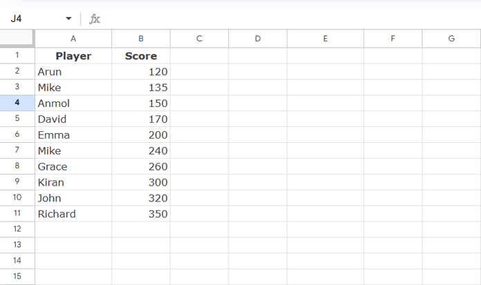
In cell D2, enter a lookup score (e.g., 140). We’ll now find the closest match.
Find the Closest Match (Higher or Lower)
Use this formula to return the player(s) with the closest score to your lookup:
=FILTER(A2:B, ABS(B2:B-D2)=SORTN(1/(ABS(B2:B-D2)*(B2:B<>""))^-1))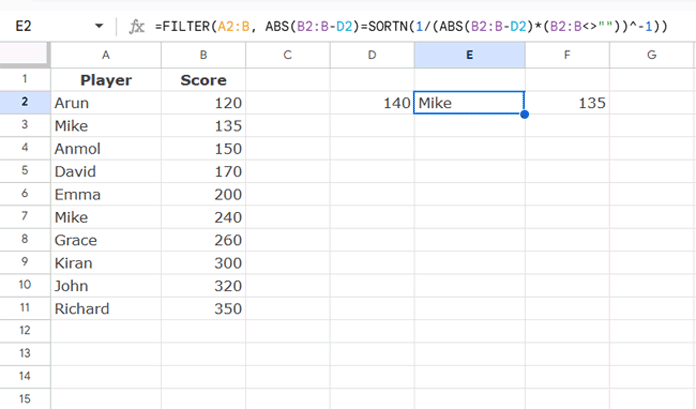
Why this works:
ABS(B2:B-D2)→ calculates the difference between each score and the lookup.SORTN(...)→ finds the minimum difference.(B2:B<>"")→ ensures empty rows are ignored.FILTER(...)→ returns the row(s) where the difference equals the minimum.
👉 Note: If two values are equally close, both will be returned. For example, if D2 = 310:
| Kiran | 300 |
| John | 320 |
If you want only one, wrap the formula with CHOOSEROWS:
- First row:
=CHOOSEROWS(FILTER(...), 1) - Last row:
=CHOOSEROWS(FILTER(...), -1)
Closest Match (Greater Than or Equal To)
To always return the next highest score:
=QUERY(A2:B, "select A, B where B >= "&D2&" order by B limit 1", 0)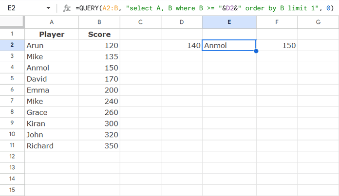
Closest Match (Less Than or Equal To)
To always return the next lowest score:
=QUERY(A2:B, "select A, B where B <= "&D2&" order by B desc limit 1", 0)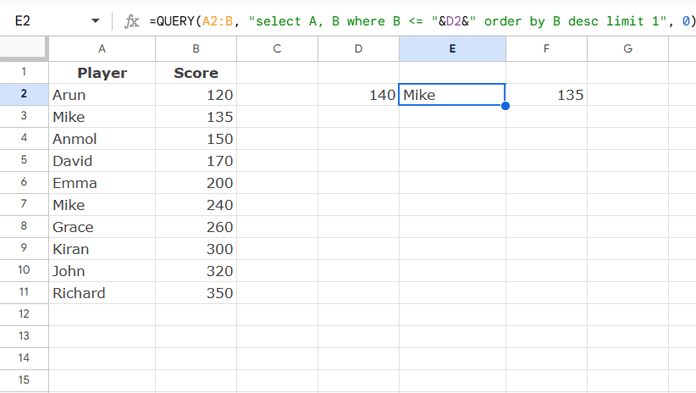
Comparison Table
| Requirement | Formula | Notes |
|---|---|---|
| Closest match (higher or lower) | =FILTER(A2:B, ABS(B2:B-D2)=SORTN(1/(ABS(B2:B-D2)*(B2:B<>""))^-1)) | May return 2 rows if equally close. Use CHOOSEROWS to pick one. |
| Closest ≥ lookup | =QUERY(A2:B, "select A, B where B >= "&D2&" order by B limit 1", 0) | Returns the next highest score. |
| Closest ≤ lookup | =QUERY(A2:B, "select A, B where B <= "&D2&" order by B desc limit 1", 0) | Returns the next lowest score. |
FAQs
Q. What happens if the lookup value is smaller than the minimum score?
- The “less than or equal to” formula will return nothing.
- The “greater than or equal to” formula will return the smallest value.
Q. What happens if the lookup value is greater than the maximum score?
- The “greater than or equal to” formula will return
#N/A. To avoid this, wrap the formula withIFNA(). - The “less than or equal to” formula will return the largest value.
Related Tutorials
- Lookup Earliest Dates in Google Sheets in a List of Items
- How to Lookup Latest Dates in Google Sheets
- Retrieve the Earliest or Latest Entry Per Category in Google Sheets
- How to Highlight Earliest Events in Google Sheets
- VLOOKUP Last or Recent Record in Each Group – Google Sheets
- Combine Rows and Keep Latest Values in Google Sheets
- How to Highlight the Latest N Values in Google Sheets


