You can use the ABS function in Google Sheets to get the absolute (modulus) value of a number. The absolute value of a number is its distance from 0 (zero) and is therefore always nonnegative.
For example, the ABS of the number -50, as well as the number 50, is 50.
ABS values can be used in problems involving distance, but they can also be used in logical tests in spreadsheets. For example, you can use the ABS function to test a column to identify the rows with values that are not equal to 0. I will provide an example of this later in this tutorial.
How to Use the ABS Function in Google Sheets: Syntax and Arguments
Syntax:
ABS(value)Argument:
value : The number to get the absolute (modulus) value of.
How to use the ABS function in Google Sheets:
You can either hardcode the value within the function or refer to a cell. Here are some examples of formulas that use hardcoded values:
=ABS(-25) // returns 25
=ABS(0) // returns 0
=ABS(25) // returns 25
You can also enter the values -25, 0, and 25 in cells A1, A2, and A3, respectively, and use the following formulas:
=ABS(A1) // returns 25
=ABS(A2) // returns 0
=ABS(A3) // returns 25
The ABS function in Google Sheets converts negative values to positive values and leaves other values unchanged. It can also be used to return the absolute values of the numbers in a range or array.
=ARRAYFORMULA(ABS(B2:B5))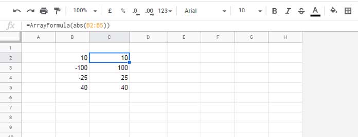
Conditional Absolute in Google Sheets
How do we do a conditional absolute in Google Sheets?
There are many ways to do this, depending on the data type you want to handle. Mostly, you can use an IF logical test.
I want to convert the numbers in C2:E9 to absolute if the corresponding values in B2:B9=”y”. The following formula does that.
=ARRAYFORMULA(IF(B2:B9="y",ABS(C2:E9),C2:E9))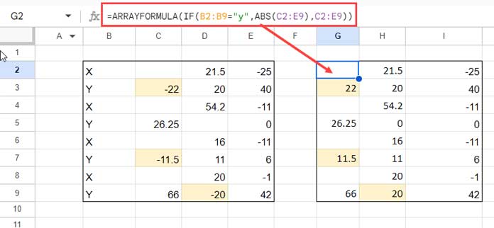
The IF function tests the condition B2:B9="y". If the condition is true, the function returns the absolute value of the corresponding cell in the range C2:E9. Otherwise, the function returns the original value of the cell in the range C2:E9.
How to Use ABS and SIGN to Find if a Value Is Not Equal to 0 in Google Sheets
With the help of an OR logical test, we can find whether a value is not equal to 0 in Google Sheets. For example, if the value is in cell A1, the following OR formula will return TRUE if the number is not equal to 0, else FALSE:
=OR(A1>0,A1<0)However, this formula will not work with an array of values in Google Sheets. For example, it will not work if you want to test all the values in column A.
To test an array of values, you can use the following formula:
=ARRAYFORMULA((A1:A>0)+(A1:A<0))This formula uses the ARRAYFORMULA function to apply the formula to all the cells in the range A1:A simultaneously. The (A1:A>0) and (A1:A<0) parts of the formula return 1 (TRUE) if the values in the range are greater than 0 or less than 0, respectively.
However, we can also replace this formula with the following combination of the ABS and SIGN functions:
=ARRAYFORMULA(ABS(SIGN(A1:A)))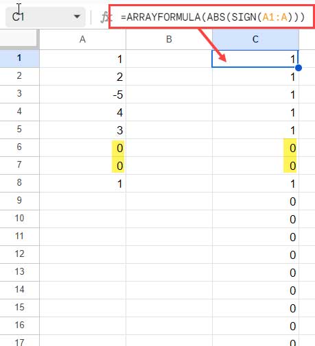
The SIGN function in Google Sheets returns -1 if the number is negative, 1 if the number is positive, and 0 if the number is zero. The ABS function returns the absolute value of a number.
Therefore, the above ABS and SING combo formula will return 1 if any of the values in the range A1:A are not equal to 0, else 0.
Additional Tip
If you want to remove the trailing zeros from the above result, because of the blank rows in the array, you can use the following formula:
=ARRAYFORMULA(LET(range,A1:A,test,ABS(SIGN(A1:A)),IF(range="",,test)))The LET function allows you to assign names to expressions so that you can reuse them in the same formula. In this case, we are using it to assign the name range to the range A1:A and the name test to the expression ABS(SIGN(A1:A)).
The IF function then evaluates if the value in the current cell in the range range is empty. If it is, the function returns an empty string. Otherwise, the function returns the value of the expression test.
The ARRAYFORMULA function then applies the formula to all the cells in the range range simultaneously.
How the ABS Function is Used in Financial Calculations
Some of the functions in Google Sheets will return negative values by default, especially those related to cash outflow. For example, the PMT function, which calculates loan payments, returns a negative value.
Calculate the loan payment and return the absolute value:
=ABS(PMT(5%/12,36,35000))In this formula, the annual interest rate of the loan is 5%, the loan period is 36 months (3 years), and the loan amount is $35,000.00. The formula would return the monthly payment value of $1,048.98.
If you want, you can replace the ABS function with the - sign in this financial calculation, which is more common.
=-pmt(5%/12,36,35000)How to Use ABS with MIN/MAX Functions to Find Absolute Minimum and Maximum
If you want to find the minimum or maximum of two values, ignoring their signs in Google Sheets, you can use the ABS function with the MIN and MAX functions.
Sample Data:
| A | B | C | D | |
| 1 | Purchase | Sales | Absolute MIN | Absolute MAX |
| 2 | -1200 | 1250 | 1200 | 1250 |
| 3 | -300 | 280 | 280 | 300 |
Formulas:
- Min Formula in C2: This formula returns the absolute minimum value of the purchase and sales values in cells A2 and B2.
=ARRAYFORMULA(MIN(ABS(A2:B2)))- Min formula in C3: This formula returns the absolute minimum value of the purchase and sales values in cells A3 and B3.
=ARRAYFORMULA(MIN(ABS(A3:B3)))- Max Formula in D2: This formula returns the absolute maximum value of the purchase and sales values in cells A2 and B2.
=ARRAYFORMULA(MAX(ABS(A2:B2)))- Max Formula in D3: This formula returns the absolute maximum value of the purchase and sales values in cells A3 and B3.
=ARRAYFORMULA(MAX(ABS(A3:B3)))In the sample data above, the ABS function is used to convert the negative purchase values to positive values. The MIN and MAX functions are then used to find the absolute minimum and maximum values of the purchase and sales values.
The results of the formulas are shown in columns C and D.


