The SIGN function is a perfect example of how a tiny function can dramatically improve your complex formulas in Google Sheets. Its primary role is to return the sign of a number, as described below:
- 1: If the number is positive.
- -1: If the number is negative.
- 0: If the number is zero.
This makes the SIGN function particularly useful in decision-making processes where the “direction” of a value matters. You can also use it in logical operations within complex formulas. I’ll provide a few examples after introducing the syntax, which is quite simple to follow.
Syntax and Basic Examples
Syntax:
SIGN(value)- value: The value whose sign is to be returned. This determines the numeric polarity.
Example:
The following formula returns:
- -1 if the value in cell
A1is less than 0. - 1 if it is greater than 0.
- 0 if it equals 0.
=SIGN(A1)If you apply the formula to a range, wrap it with the ARRAYFORMULA function:
=ARRAYFORMULA(SIGN(A1:A10))Note: If a referenced cell is empty, the formula will return 0.
SIGN Function for Logical Tests
The SIGN function can be used as an alternative to the OR logical test. Here’s how:
Example 1: Replacing the OR Function
The following OR formula checks if either A1 or B1 is greater than 50. It returns TRUE if either condition is met, and FALSE otherwise:
=OR(A1>50, B1>50)TRUE and FALSE are Boolean values represented as 1 and 0, respectively.
You can replace this with the SIGN function as follows:
=SIGN((A1>50)+(B1>50))This formula will return 1 if either condition is true and 0 otherwise. Without SIGN, the formula would return 2 if both conditions are true, as it sums up the Boolean values (1+1=2). The SIGN function normalizes this to 1, equivalent to TRUE.
For example, you can replace this formula:
=IF(OR(A1>50, B1>50), "Pass", "Fail")With:
=IF(SIGN((A1>50)+(B1>50)), "Pass", "Fail")Why use the SIGN function over OR?
The SIGN function can handle ranges and return expanded results, while OR cannot. For instance, this formula won’t work row by row:
ArrayFormula(IF(OR(A1:A5>50, B1:B5>50), "Pass", "Fail"))But this SIGN formula can:
=ArrayFormula(IF(SIGN((A1:A5>50)+(B1:B5>50)), "Pass", "Fail"))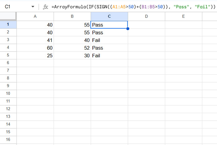
Example 2: Using SIGN in SUMPRODUCT
You can also apply the same logic in SUMPRODUCT.
For example, suppose:
- Column A contains student names.
- Columns B and C contain their scores from two attempts.
- Column D contains their total score.
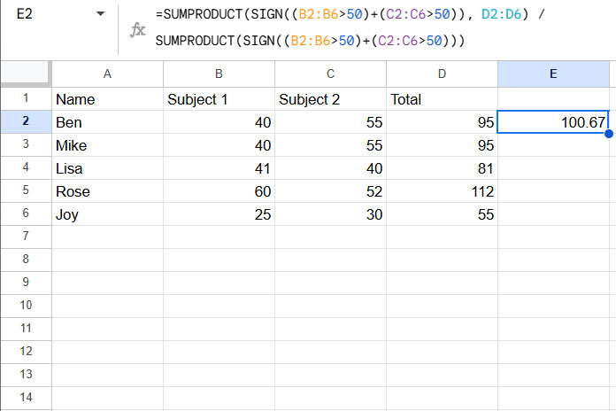
To calculate the average score of students who passed, use the following formulas:
Total score of passed students:
=SUMPRODUCT(SIGN((B2:B6>50)+(C2:C6>50)), D2:D6)Count of students who passed:
=SUMPRODUCT(SIGN((B2:B6>50)+(C2:C6>50)))Average score of passed students:
=SUMPRODUCT(SIGN((B2:B6>50)+(C2:C6>50)), D2:D6) / SUMPRODUCT(SIGN((B2:B6>50)+(C2:C6>50)))Related: How to Use OR Condition in SUMPRODUCT in Google Sheets.
SIGN Function in MMULT for Summation
The MMULT function is commonly used for matrix multiplication in Google Sheets. However, you can use it for summing each row or column dynamically, without requiring a LAMBDA function.
Here’s how the SIGN function helps:
Example:
Consider the following table in A1:C4:
| 50 | 15 | 20 |
| 25 | 20 | 30 |
| 40 | 30 | 40 |
| 50 | 60 | 50 |
To calculate the total of each column, use this formula in A5:
=ArrayFormula(MMULT(SIGN(TOROW(A1:A4)), A1:C4))SIGN(TOROW(A1:A4))generates a horizontal array of 1s matching the number of rows in the matrix.
To calculate the total of each row, use this formula in D1:
=ArrayFormula(MMULT(A1:C4, SIGN(TOCOL(A1:C1))))SIGN(TOCOL(A1:C1))generates a vertical array of 1s matching the number of columns in the matrix.
Wrap-Up
The SIGN function in Google Sheets offers a range of applications, from basic use cases to advanced logic in formulas. You can even use it in conditional formatting or logical tests with functions like FILTER, SUMIF, and AVERAGEIF.
Master the examples above, and you’ll unlock the full potential of this simple yet powerful function.


