The PMT function in Google Sheets helps calculate the periodic payments for a loan or an annuity. Whether you’re working with a loan or an investment, the PMT formula can be used to determine consistent periodic payments based on a constant interest rate and loan term.

In this guide, you’ll learn how to use the PMT function with examples and formulas. By the end, you’ll also find a link to a simple EMI calculator I’ve created in Google Sheets, which you can use for educational purposes.

Key Points about the PMT Function:

• It calculates both principal and interest in the periodic payments.
• The payment result doesn’t include taxes, insurance, or fees that may be part of a real-life loan.

PMT Function Syntax

Let’s start with the syntax of the PMT function:

PMT(rate, number_of_periods, present_value, [future_value], [end_or_beginning])

Now, let’s break down the arguments:

• rate (APR): The annual interest rate divided by the number of periods (months, quarters, etc.).
• number_of_periods (NPER): The total number of payments for the loan or investment.
• present_value (PV): The current value or principal amount of the loan or investment.
• future_value (FV): Optional; it’s 0 by default. It represents the desired future value at the end of the term.
• end_or_beginning: Optional; it’s 0 by default. It specifies whether payments are made at the end (0) or beginning (1) of each period.

Example 1: Calculating Monthly Payments for a Car Loan

Let’s use the PMT function to calculate monthly payments for a $35,000 car loan at 5% annual interest, with a loan term of 72 months. Assume the following input data:

• Annual Interest Rate (APR): 5% (cell C3)
• Loan Term in Months: 72 (cell C4)
• Loan Amount (PV): $35,000 (cell C5)

Here’s the formula to calculate the monthly payment:

=PMT(C3/12, C4, C5)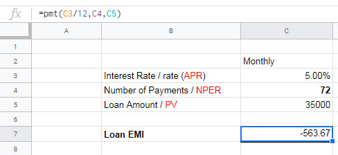

Since the interest rate is annual, we divide it by 12 to convert it to a monthly rate. The result will be a negative value because it represents an outflow (payment). To display the payment as a positive value, modify the formula like this:

=-PMT(C3/12, C4, C5)

You would use the following formula if you make payments at the beginning of each month:

=-PMT(C3/12, C4, C5, 0, 1)

Example 2: Calculating Quarterly Payments

Now, let’s calculate quarterly payments using the same car loan example. The key difference is that we divide the interest rate by 4 (for quarters) and adjust the loan term to reflect quarterly periods:

Number of Quarters: 6 years × 4 quarters = 24 (update cell C4)

Formula:

=PMT(C3/4, C4, C5)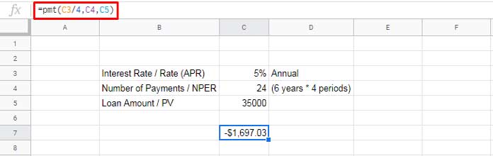

Example 3: Calculating Yearly Payments

For yearly payments, the formula is even simpler. Since the interest rate is already annual, no division is needed:

=PMT(C3, C4, C5)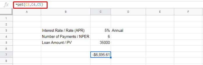

Using the Future Value (FV) Argument

Suppose you want to know how much you need to invest monthly to accumulate $25,000 in 8 years, given an 8.5% annual interest rate. You will receive a future value (FV) of $25,000 by making monthly payments.

Formula:

=PMT(8.5%/12, 8*12, 0, 25000) // returns $182.72

The result tells you that if you deposit approximately $182.72 monthly, you will accumulate $25,000 by the end of 8 years.

Creating an EMI Calculator in Google Sheets

Now, let’s create an EMI calculator using the PMT function. Here are the input values:

• Loan Amount (cell C2): $85,000
• Interest Rate (Annual) (cell C3): 4%
• Loan Tenure (cell C4): 30 (years or months, based on your selection)

The formula used in the calculator is:

=-PMT(IFS(D4="Year",C3,D4="Month",C3/12), C4, C2)

EMI Calculator

This formula is slightly different because it includes the IFS function to handle the loan tenure as either years or months.

Explanation of Formula Logic:

• The IFS function determines whether the loan tenure is entered in years or months and adjusts the calculation accordingly.

With this approach, you can calculate the EMI for home, car, or personal loans with flexible input formats.

That’s it! I hope this guide helps you understand how to use the PMT function and create an EMI calculator in Google Sheets. Happy calculating!