Want to build a completely custom, dynamic unit converter in Google Sheets? Whether you need to convert metrics for weight, distance, temperature, or volume, the native CONVERT function makes it incredibly easy.
Instead of hardcoding individual conversion formulas, this guide will show you how to make a unit converter in google sheets using dynamic drop-down lists.
This tutorial offers a free downloadable unit calculator template, helping you master the CONVERT function and build your own custom calculator from scratch.
How to Use the Unit Converter Template
Using the automated unit converter is simple and intuitive. Follow these quick steps to perform any conversion instantly:
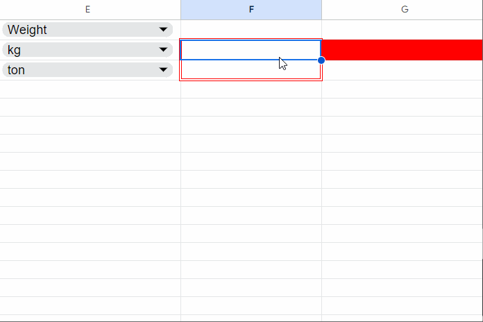
- Select a Category: Choose one of the 13 available measurement categories from the drop-down menu in cell E1 (such as Weight, Distance, Temperature, or Volume).
- Choose Your Units: Select your starting unit code in cell E2 (“Convert From”) and your target unit code in cell E3 (“Convert To”).
- Enter Your Value: Type the number you want to convert into cell F2 (or F3). The template will automatically calculate the result and display it cleanly in cell G2.
Bonus Feature: If you are unsure what a specific shortcode means (like “lbm” or “Pa”), you will find a dynamic abbreviation lookup table built into the template directly below the converter to show you the full unit descriptions instantly.
Now that you know how to use the tool, let’s pull back the curtain to understand how the native CONVERT function works under the hood, and how you can build this dynamic calculator yourself.
How to Use the CONVERT Function in Google Sheets
The core of the unit converter is the native CONVERT function. It is straightforward to use once you understand its layout.
Syntax:
=CONVERT(value, start_unit, end_unit)- value – The numeric value you want to convert (this can be a raw number or a cell reference).
- start_unit – The current measurement unit of your starting value. This must be wrapped in quotation marks if entered directly into the formula (e.g., “ton”).
- end_unit – The target measurement unit you want to convert to (e.g., “kg”).
Example:
=CONVERT(1000, "kg", "ton")Crucial Rule: Your start_unit and end_unit must belong to the exact same measurement category. For example, you cannot use CONVERT to cross-reference a unit from the “Weight” category with a unit from the “Distance” category. Doing so will result in an #N/A error with the message: “Error: Invalid units for conversion.”
In our dynamic unit converter template, we automate this process using cell references instead of hardcoded unit names. The formula dynamically reads the category selected via the drop-down menu in cell E1. It then looks at the corresponding starting and target units chosen in cells E2 and E3, which are populated using dependent drop-downs to prevent errors. Finally, it pulls the raw value to convert straight from cell F2 or F3 depending on which field you enter your data into.
Categories and Units for the CONVERT Function
Here are the available conversion units for the CONVERT function.
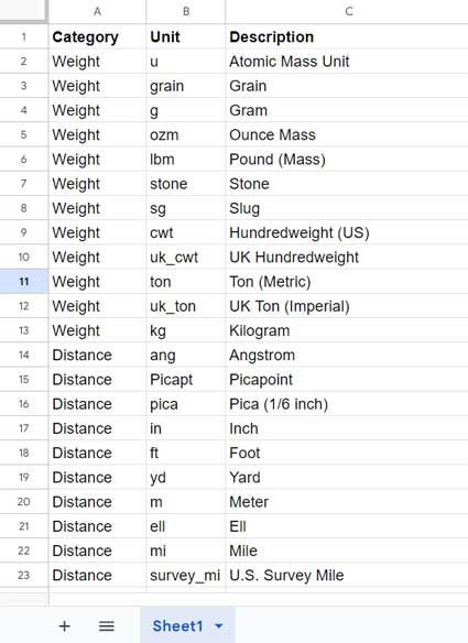
Weight
| unit | description |
|---|---|
| u | Atomic Mass Unit |
| grain | Grain |
| g | Gram |
| ozm | Ounce Mass |
| lbm | Pound (Mass) |
| stone | Stone |
| sg | Slug |
| cwt | Hundredweight (US) |
| uk_cwt | UK Hundredweight |
| ton | Ton (Metric) |
| uk_ton | UK Ton (Imperial) |
| kg | Kilogram |
Distance
| unit | description |
|---|---|
| ang | Angstrom |
| Picapt | Picapoint |
| pica | Pica (1/6 inch) |
| in | Inch |
| ft | Foot |
| yd | Yard |
| m | Meter |
| ell | Ell |
| mi | Mile |
| survey_mi | U.S. Survey Mile |
| Nmi | Nautical Mile |
| ly | Light Year |
| parsec | Parsec |
Time
| unit | description |
|---|---|
| sec | Second |
| min | Minute |
| hr | Hour |
| day | Day |
| yr | Year |
Pressure
| unit | description |
|---|---|
| Pa | Pascal |
| mmHg | Millimeter of Mercury |
| Torr | Torr |
| psi | Pounds per Square Inch |
| atm | Atmosphere |
Force
| unit | description |
|---|---|
| dyn | Dyne |
| pond | Pond |
| N | Newton |
| lbf | Pound-force |
Energy
| unit | description |
|---|---|
| eV | Electron Volt |
| e | Erg |
| J | Joule |
| flb | Foot-Pound (or Foot-Pound Force) |
| c | Thermodynamic Calorie |
| cal | IT Calorie |
| BTU | British Thermal Unit |
| Wh | Watt-Hour |
| HPh | Horsepower-Hour |
Power
| unit | description |
|---|---|
| W | Watt |
| PS | Pferdestärke (Metric Horsepower) |
| HP | Horsepower |
Magnetism
| unit | description |
|---|---|
| ga | Gauss |
| T | Tesla |
Temperature
| unit | description |
|---|---|
| C | Celsius |
| F | Fahrenheit |
| K | Kelvin |
| Rank | Rankine |
| Reau | Réaumur |
Volume
| unit | description |
|---|---|
| ang^3 | Cubic Angstrom |
| Picapt^3 | Cubic Picapoint |
| tsp | Teaspoon |
| tspm | Teaspoon Metric |
| tbs | Tablespoon |
| in^3 | Cubic Inch |
| oz | Ounce (Fluid) |
| cup | Cup |
| pt | Pint |
| uk_pt | UK Pint |
| qt | Quart |
| l | Liter |
| uk_qt | UK Quart |
| gal | Gallon |
| uk_gal | UK Gallon |
| ft^3 | Cubic Foot |
| bushel | Bushel |
| barrel | Barrel |
| yd^3 | Cubic Yard |
| m^3 | Cubic Meter |
| MTON | Measurement Ton |
| GRT | Gross Register Ton |
| mi^3 | Cubic Mile |
| Nmi^3 | Cubic Nautical Mile |
| ly^3 | Cubic Light-Year |
Area
| unit | description |
|---|---|
| ang^2 | Square Angstrom |
| Picapt^2 | Square Picapoint |
| in^2 | Square Inch |
| ft^2 | Square Foot |
| yd^2 | Square Yard |
| m^2 | Square Meter |
| ar | Are |
| Morgen | Morgen |
| uk_acre | UK Acre |
| us_acre | US Acre |
| ha | Hectare |
| mi^2 | Square Mile |
| Nmi^2 | Square Nautical Mile |
| ly^2 | Square Light Year |
Information
| unit | description |
|---|---|
| bit | Binary Digit |
| byte | 8 Bits |
Speed
| unit | description |
|---|---|
| m/hr | Meters per Hour |
| mph | Miles per Hour |
| kn | Knots |
| admkn | Admiralty Knots |
| m/s | Meters per Second |
Steps to Make a Unit Converter in Google Sheets
Follow these step-by-step instructions to build the fully automated unit converter from scratch.
Phase 1: Setting Up the Database
First, create your master reference list in columns A, B, and C. Label cells A1:C1 as “Category”, “Unit”, and “Description”. You can use the comprehensive unit tables provided above to populate rows 2 and downward.
Phase 2: Building the Dependent Drop-Down Menus
Next, follow these steps to create your interactive menus:
- Select cell E1 (this will be your Category selector).
- Click Insert > Drop-down to open the Data Validation sidebar.
- In the Criteria menu, select “Drop-down (from a range)”.
- Enter A2:A in the range field and click Done.
- Navigate to cell D1 and enter the following VSTACK and FILTER formula to build a dynamic helper column:
=VSTACK("Helper", FILTER(B2:B, A2:A=E1)) - Select cell E2 (your “From Unit” selector).
- Click Insert > Drop-down, choose “Drop-down (from a range)”, and enter D2:D as the range. Click Done.
- Copy cell E2 and paste it into cell E3 to create your “To Unit” selector.
Phase 3: Adding the Multi-Directional Conversion Formula
To make the converter incredibly flexible, we want it to work regardless of whether you type your number into cell F2 or cell F3. If you type a value in F2, it converts from the unit in E2 to E3. If you type a value in F3, it reverses and converts from E3 to E2.
- Navigate to cell G2.
- Paste the following master formula:
=IFERROR(CONVERT(SORTN(F2:F3), FILTER(E2:E3, F2:F3), FILTER(E2:E3, F2:F3="")))
Now, simply enter the number you want to convert into either cell F2 or F3, and cell G2 will instantly output the mathematically precise result.
Phase 4: Adding Dynamic Unit Description Lookups (Optional)
To make the converter user-friendly, we can display the full name of the selected unit abbreviations (like changing “lbm” to “Pound (Mass)”).
- Navigate to cell F7 and enter this formula to display the full “From Unit” description:
=IFNA(E2&" ("&XLOOKUP(E2, B2:B, C2:C)&")") - Navigate to cell F8 and enter this formula to display the full “To Unit” description:
=IFNA(E3&" ("&XLOOKUP(E3, B2:B, C2:C)&")")
Formula Breakdown: How the Array Logic Works
The master formula uses advanced array filtering to dynamically swap the arguments inside the CONVERT function based on where you enter your data. Here is exactly how it satisfies the three required arguments:
- value:
SORTN(F2:F3)This looks at the range F2:F3 and isolates whichever cell contains your raw number, passing it directly to the function. - start_unit:
FILTER(E2:E3, F2:F3)This filters your unit selections in E2:E3 and returns the starting unit code associated with the cell where you actively typed a number. - end_unit:
FILTER(E2:E3, F2:F3="")This filters E2:E3 for the empty input cell, identifying it as your target destination and pulling the correct target unit code.
Wrapping the entire string in IFERROR ensures that your spreadsheet displays a clean blank cell or custom text instead of throwing a generic error when the input cells are empty.
Unit Descriptions: XLOOKUP and IFNA
The lookup formulas in F7 and F8 combine text joining (&) with XLOOKUP to scan your master database in columns B and C. It matches the short code from your drop-down (E2 or E3) and pairs it with its full description.
Wrapping the formula in IFNA prevents the sheet from displaying ugly #N/A errors when the unit drop-downs are left blank, keeping your calculator template looking professional and clean.


