To look up the latest value, we can use the function LOOKUP. It’s available in both Excel and Google Sheets.
Another powerful alternative is XLOOKUP in Google Sheets. This function is also available in modern versions of Excel (generally Office 365 with a subscription).
What is the latest value then?
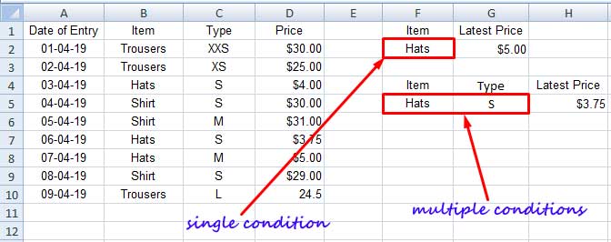
Assume an item repeats multiple times in a column. For example, the item “Hats” (please refer to the below screenshot) repeats in the cells B4, B7, and B8. You can consider the values in row # 8 as the latest values of this keyword.
Note: If you have a date column, the dataset should be sorted based on this column in ascending order.
How to Lookup Latest Value in Excel
In the above sample dataset (A1:D10), I want to search for the item “Hats” in cells B2:B10 and return its latest “Price” from the range D2:D10.
I’ve entered the criterion “Hats” in cell F2. Here is the LOOKUP formula that I’ve used in cell G2 to return the latest value (Price) of “Hats”.
=LOOKUP(2, 1/(B2:B10=F2), D2:D10)You should enter it as an array formula by pressing Ctrl+Shift+Enter (CSE) if you are not using Excel versions that support dynamic array formulas.
Formula Breakdown
First, let’s review the LOOKUP Function Syntax:
=LOOKUP(lookup_value, lookup_vector, result_vector)lookup_value:
In our example, 2 is the lookup_value, also known as the search key. The LOOKUP searches for this value in the lookup_vector (B2:B10).
Why are you using 2 as the search key instead of “Hats” in cell F2?
Just keep reading to understand why I have used that number instead of the actual search key, which is “Hats”.
lookup_vector:
The lookup_vector is the range to search for the lookup_value (“Hats”). It’s actually B2:B10. However, I have used a virtual lookup_vector as follows:
1/(B2:B10=F2)To understand what this formula returns, you must enter this formula as an Array Formula using Ctrl+Shift+Enter.
As an example, I am entering this formula in cell E2 as an array formula.
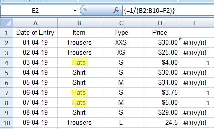
To do this, first select the result range E2:E10, then enter the formula in E2, and finally press the CSE shortcut keys.
We won’t use it anywhere in our LOOKUP formula. This is just to help you understand what it returns. This formula returns 1 wherever the keyword, which is “Hats”, matches.
result_vector:
It is the range D2:D10, which contains the prices of items.
How does the LOOKUP formula work?
Please note that our search key is the number 2. The LOOKUP function will search for this key in the lookup_vector range. That range now only contains the error values and the number 1.
Since the LOOKUP formula can’t find the lookup_value in this column, it matches the largest value in the lookup_vector that is less than or equal to the lookup_value (2).
There are multiple occurrences of 1 in the lookup_vector, so the last row or column in the result_vector corresponding to the matching value is returned.
Find the Latest Value Based on Multiple Conditions in Excel
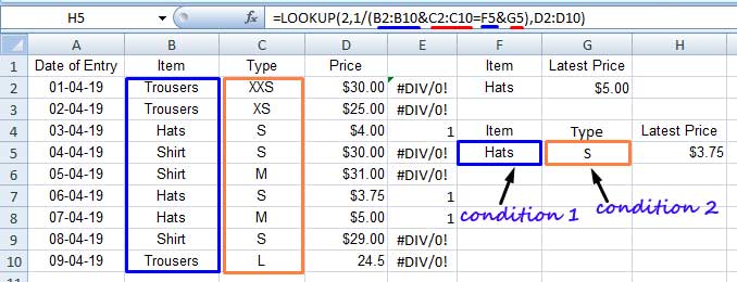
This time, I don’t want the latest price of the item “Hats”. Instead, what I want is the latest price of the item “Hats”, of which the size is “S”. These criteria are in cells F5 and G5 respectively.
The following Excel LOOKUP formula handles multiple (two) search keys.
=LOOKUP(2, 1/(B2:B10&C2:C10=F5&G5), D2:D10)The lookup_vector and lookup_value are both combined ranges.
These changes will help you look up the latest value based on multiple conditions in Excel.
How to Lookup Latest Value in Google Sheets
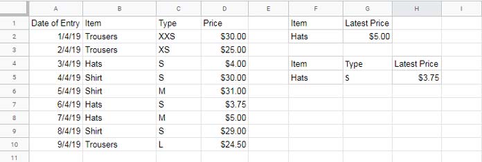
To look up the latest value in Google Sheets, you can use the same Excel formulas provided above, both for single and multiple conditions. However, you must include the ARRAYFORMULA function with the Google Sheets LOOKUP formulas. This might cause some confusion for Excel users transitioning to Google Sheets.
Single Condition:
=ArrayFormula(LOOKUP(2, 1/(B2:B10=G2), D2:D10))Multiple Conditions:
=ArrayFormula(LOOKUP(2, 1/(B2:B10&C2:C10=G5&H5), D2:D10))XLOOKUP: An Alternative Solution
If you’re using Google Sheets, the easiest way to look up the latest values is using XLOOKUP.
Single Criteria:
=XLOOKUP(F2, B2:B10, D2:D10, "", 0, -1)Where F2 is the search key, B2:B10 is the lookup range, and D2:D10 is the result range. 0 represents an exact match and -1 indicates searching from bottom to top.
Regarding multiple search keys, you can follow the same earlier approach, combining criteria as well as lookup ranges.
=ArrayFormula(XLOOKUP(F5&G5, B2:B10&C2:C10, D2:D10, "", 0, -1))What about Excel?
If your Excel supports XLOOKUP and dynamic array formulas, you can use the above formulas. In the second formula, you should remove the ArrayFormula function.


