If you want to use the Excel XMATCH function alternatives in Google Sheets, you are in the right spot.

You can get the alternative formulas to almost all the XMATCH variations here in this post.

At the time of writing this post, the XMATCH function is not available in Google Sheets. What about alternatives?

Update: Learn the new XMATCH function here – XMATCH Function in Google Sheets (Formula Examples).

Of course, we can use alternative formulas to meet our XMATCH requirement in Google Sheets.

If you haven’t heard about this function name so far, it’s a Microsoft Excel 365 function to get the relative position of values in a vertical or horizontal array/range.

We can use the Google Sheets MATCH function as an alternative to the XMATCH function in Excel. But as a combination formula only.

So learning MATCH is not enough!

Then?

You must have some basic knowledge in using a few of the Google Sheets functions to use it as an alternative to the XMATCH.

But don’t worry. I will help you use the MATCH function as an alternative to the XMATCH function.

You can bookmark this page for future reference.

XMATCH Function Alternatives in Google Sheets

We usually use the XMATCH in Excel for the following purposes.

Please pay special attention to the points noted in the last two columns in the above table.

When you write XMATCH function alternative formulas in Google Sheets, you must consider them.

Also, there is one more important thing to consider.

What is that?

The formulas should not only work with numbers but also with text strings.

I have ensured that my formula works in both cases.

But you should test them thoroughly on your end before start using in your Sheets.

Below you can find the six XMATCH formulas to use in the above different scenarios (Sr. No. 1 to 6 in the table) in Excel and its alternatives in Google Sheets.

Example 1 – Relative Positions in Numeric Array

I have the following vertical array in Google Sheets in which we are going to test six XMATCH function alternative formulas.

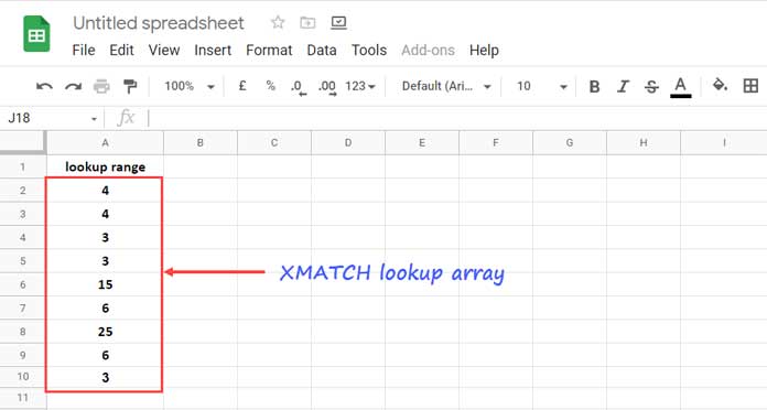
The lookup range/array is A2:A10, and it contains numeric values.

You can keep the values as it’s. I mean no need to sort the range.

The following formulas are as per the above table_1 (match type and response to duplicates) order.

Six XMATCH Function Alternative Formulas and Their Real Excel Counterparts

In the following formulas, you must replace “Lookup_Value” with the original value to match.

Note:- The term first/last values denote how the formula responds to duplicates.

1. Exact match the first value.

Google Sheets Formula:

=match(Lookup_Value,A2:A10,0)

Excel Formula:

=XMATCH(Lookup_Value,A2:A10,0,1)

2. Exact match the last value.

Google Sheets Formula:

=ArrayFormula(match(1,1/(A2:A10=Lookup_Value),1))

Excel Formula:

=XMATCH(Lookup_Value,A2:A10,0,-1)

In the below formulas, I’ll use two additional functions, and they are SORTN and FILTER.

3. Exact match the first value or the next (first) largest value.

Google Sheets Formula:

=ArrayFormula(match(1,1/(A2:A10=sortn(filter(A2:A10,A2:A10>=Lookup_Value))),-1))

Excel Formula:

=XMATCH(Lookup_Value,A2:A10,1,1)

4. Exact match the last value or the next (last) largest value.

Google Sheets Formula:

=ArrayFormula(match(1,1/(A2:A10=sortn(filter(A2:A10,A2:A10>=Lookup_Value))),1))

Excel Formula:

=XMATCH(Lookup_Value,A2:A10,1,-1)

5. Exact match the first value or the next (first) smallest value.

Google Sheets Formula:

=ArrayFormula(match(1,1/(A2:A10=sortn(filter(A2:A10,A2:A10<=Lookup_Value),1,0,1,0)),-1))

Excel Formula:

=XMATCH(Lookup_Value,A2:A10,-1,1)

6. Exact match the last value or the next (last) smallest value.

Google Sheets Formula:

=ArrayFormula(match(1,1/(A2:A10=sortn(filter(A2:A10,A2:A10<=Lookup_Value),1,0,1,0)),1))

Excel Formula:

=XMATCH(Lookup_Value,A2:A10,-1,-1)

The above are the alternatives to the XMATCH function in Google Sheets.

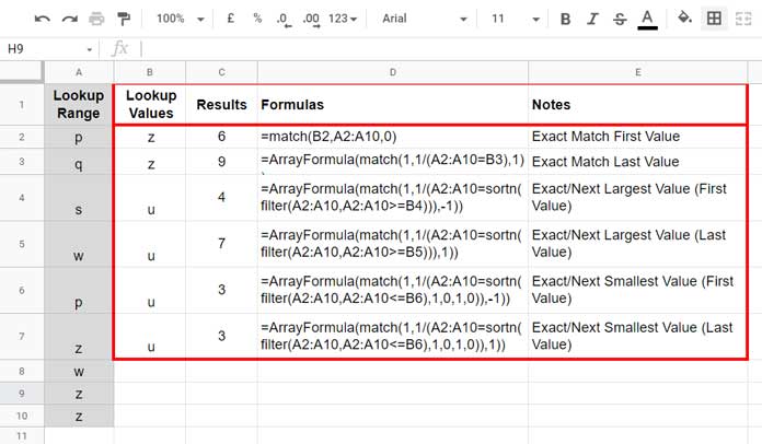
Example 2 – Relative Positions in Text Array

Since all the above six formulas work equally well in date and text array, I am not repeating them.

Instead, here is a screenshot in which you can see the formulas and their result.

I have used the same lookup range/array. So you can use the above same formulas.

If you are an Excel user and want to use the original XMATCH formulas, you can use the above six corresponding formulas.

That’s all about XMATCH function alternatives in Google Sheets.

Thanks for the stay. Enjoy!

Additional Resources:

• How to Find the Last Matching Value in Google Sheets.
• Vlookup to Find Nth Occurrence in Google Sheets [Dynamic Lookup].
• Lookup Last Partial Occurrence in a List in Google Sheets.
• Lookup to Find the Last Occurrence of Multiple Criteria in Google Sheets.
• Highlight Nth Occurrence of a Value in Google Sheets.