XLOOKUP Alternatives in Google Sheets

Introduction

The XLOOKUP function, a modern lookup feature in Excel, is now also available in Google Sheets. However, exploring alternative formulas can help you understand the versatility of Google Sheets and allow you to perform similar lookups.

Although many Google Sheets users managed without XLOOKUP by using workarounds, these alternatives offer powerful options to replicate much of XLOOKUP’s functionality.

This guide provides several alternative formulas, covering exact matches, multiple returns, and advanced match modes.

Note: For simplicity, stick with XLOOKUP, as it makes lookups much easier.

XLOOKUP Formula Alternatives: Basic Exact Match Lookups

Below, we cover several alternatives to XLOOKUP for exact match lookups in Google Sheets.

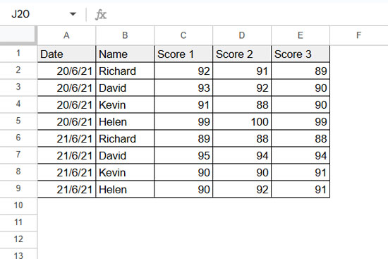
Sample Data

Use the “Basic” tab in the Example Sheet to follow along. Copy the sheet to your Google Drive to practice each example.

Sample Data

1. Exact Match: Retrieve Value Based on Lookup

Task

Find the exact match of “David” in column B and return the score from column E.

Formula Comparison

XLOOKUP Formula:
=XLOOKUP("David", B2:B9, E2:E9)
Alternative with VLOOKUP:
=VLOOKUP("David", {B2:B9, E2:E9}, 2, 0)

2. Reverse Lookup: Retrieve Value from a Different Column

Task

Look up the name “David” in column B and return the corresponding date from column A.

Formula Comparison

XLOOKUP Formula:
=XLOOKUP("David", B2:B9, A2:A9)
Alternative with VLOOKUP:
=VLOOKUP("David", {B2:B9, A2:A9}, 2, 0)

Tip: The result might display as a serial number if the cell is not formatted as a date. To adjust, go to Format > Number > Date.

3. Return Multiple Columns in Result Array

Task

Return multiple columns (C to E) for the lookup value “David” in column B.

Formula Comparison

XLOOKUP Formula:
=XLOOKUP("David", B2:B9, C2:E9)
Alternative with ArrayFormula and VLOOKUP:
=ArrayFormula(VLOOKUP("David", {B2:B9, C2:E9}, {2,3,4}, 0))

4. Lookup with Multiple Values

Task

Retrieve scores for both “David” and “Helen” in column B.

Formula Comparison

XLOOKUP Formula:
=ArrayFormula(XLOOKUP({"David"; "Helen"}, B2:B9, E2:E9))
Alternative:
=ArrayFormula(VLOOKUP({"David"; "Helen"}, {B2:B9, E2:E9}, 2, 0))

5. Combination of Multiple Lookup Values and Multiple Return Columns

Task

Return multiple columns (C to E) for “David” and “Helen” in column B.

Formula Comparison

XLOOKUP Formula (currently unavailable for 2D arrays):
Requires LAMBDA functions for 2D results.
Alternative with VLOOKUP and ArrayFormula:
=ArrayFormula(VLOOKUP({"David"; "Helen"}, {B2:B9, C2:E9}, {2,3,4}, 0))

Match and Search Modes in XLOOKUP Alternatives

XLOOKUP’s match and search modes are advanced features that make it versatile.

Below, we break down four types of match and search modes and demonstrate how to achieve them with formulas in Google Sheets.

Sample Data

The data set includes timestamps in column A, order numbers in column B, and order quantities in column C. This data can be viewed in the ‘Match and Search Modes – SMALL’ tab of the sample sheet linked above.

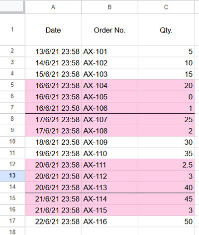
In all the following examples, the criterion will be a timestamp or date entered in cell E2.

1. Exact / Next Smallest – Last Value

Task

Return the quantity for a timestamp that either matches exactly or is the next smallest value in column A.

Formula Comparison

XLOOKUP Formula:
=XLOOKUP(E2, A2:A17, C2:C17, , -1, -1)
Alternative with VLOOKUP:
=VLOOKUP(E2, SORT({A2:A17, C2:C17}, 1, 1), 2, 1)

2. Exact / Next Smallest – First Value

Task

Return the quantity for a timestamp that matches exactly or is the next smallest, prioritizing the first occurrence.

Formula Comparison

XLOOKUP Formula:
=XLOOKUP(E2, A2:A17, C2:C17, , -1, 1)
Alternative with SORTN and VLOOKUP:
=VLOOKUP(E2, SORTN({A2:A17, C2:C17}, 9^9, 2, 1, 1), 2, 1)

3. Exact / Next Largest – Last Value

For this example, refer to the sample data in the ‘Match and Search Modes – LARGE’ tab in the sample sheet above. It’s similar to the previous sample data, with a few timestamps adjusted in column A.

Task

Find the next largest timestamp and return the last occurrence.

Formula Comparison

XLOOKUP Formula:
=XLOOKUP(E2, A2:A17, C2:C17, , 1, -1)
Alternative with IFNA, SORT, and SORTN:

=IFNA(VLOOKUP(E2, SORT({A2:A17, C2:C17, ROW(A2:A17)}, 3, 0), 2, 0),
VLOOKUP(E2, {{1/0; INDEX(SORTN(SORT({A2:A17, C2:C17, ROW(A2:A17)}, 3, 0), 9^9, 2, 1, 1), , 1)},
{INDEX(SORTN(SORT({A2:A17, C2:C17, ROW(A2:A17)}, 3, 0), 9^9, 2, 1, 1), , 2); IF(,,)}}, 2, 1))

4. Exact / Next Largest – First Value

Task

Find the next largest timestamp and return the first occurrence.

Formula Comparison

XLOOKUP Formula:
=XLOOKUP(E2, A2:A17, C2:C17, , 1, 1)
Alternative with IFNA and SORTN:

=IFNA(VLOOKUP(E2, {A2:A17, C2:C17}, 2, 0),
VLOOKUP(E2, {{1/0; INDEX(SORTN({A2:A17, C2:C17}, 9^9, 2, 1, 1), , 1)},
{INDEX(SORTN({A2:A17, C2:C17}, 9^9, 2, 1, 1), , 2); IF(,,)}}, 2, 1))

Conclusion

While XLOOKUP in Google Sheets offers powerful match and search options, these alternative formulas provide similar functionality.

In the examples above, we haven’t addressed XLOOKUP’s capabilities for wildcard matches and binary search modes.

Overall, XLOOKUP is significantly more versatile and efficient than its alternatives.