When you have empty cells scattered across a row, you may want to remove those blank cells and shift the remaining values to the left. This helps create cleaner, more structured data in Google Sheets.

While Google Sheets provides a built-in option to shift cells left, it comes with limitations. That’s why, in most cases, it’s better to use a formula-based workaround to delete empty cells and shift left in Google Sheets.

Shift Cells to the Left Using the Built-in Method

Let’s say you have data in A1:E1, and B1 and C1 are empty.

1. Select B1:C1.
2. Right-click and choose Delete cells > Delete cells and shift left.

Limitations

• This method works only when the selected cells are adjacent.
• For 2D ranges, the selection must be rectangular — all rows and columns must form a continuous block with equal dimensions.
• However, for a single row (1D), you can use “Delete cells > Shift left” even if only a part of the row is selected.

In short, this method doesn’t work well when blank cells are scattered across multiple rows or if the selection is irregular.

How Excel Handles This Better

In Excel, removing blank cells and shifting data left is much easier:

1. Select your range.
2. Go to Home > Find & Select > Go to Special > Blanks > OK.
3. Then choose Delete > Delete Cells > Shift Cells Left.

Done! Excel automatically shifts non-blank cells to the left wherever blanks are found — no formulas needed.

Remove Blank Cells and Shift Left in Google Sheets Using Formulas

Unfortunately, Google Sheets doesn’t provide a similar built-in method. But don’t worry — formulas can help you remove blank cells and shift left in Google Sheets effectively.

Note: Formula-based solutions output results in a new range. To overwrite your source data, you’ll need to copy and paste values afterward.

The benefit of using a formula, though, is that it dynamically updates. If new data is added, the formula adjusts automatically — no need for manual reprocessing.

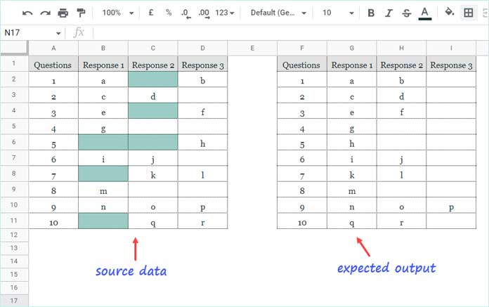
This technique is especially useful when cleaning up Form Responses, where you often get blank cells in between values.

Formula Examples to Delete Empty Cells and Shift Left in Google Sheets

Let’s say you have data in the range A2:D.

Option 1: Non-Array Formula (Manual Copy-Paste)

Insert this formula in cell F2 and drag it down:

=IFNA(FILTER(A2:D2, A2:D2 <> ""))

What it does: Filters out empty cells from each row, shifting the remaining values left.

To finalize:

1. Select the filled output range (e.g., F2:I).
2. Copy it.
3. Go to the original range (A2:D) and use Edit > Paste special > Values only.
4. Delete the formulas.

Alternatively, you can use:

=TOROW(A2:D2, 3)

This also removes blank cells and shifts remaining values left into a single row.

Option 2: Array Formula (Automatic)

To apply the logic across multiple rows, use BYROW with a LAMBDA function.

Filter-based version:

=BYROW(A2:D, LAMBDA(row, IFNA(FILTER(row, row <> ""))))

TOROW-based version:

=BYROW(A2:D, LAMBDA(row, TOROW(row, 3)))

These formulas process each row in your range and delete empty cells, shifting values left.

Conclusion

While Google Sheets lacks Excel’s flexibility in handling blank cells, formulas offer a reliable workaround to remove blank cells and shift left in Google Sheets. Whether you’re organizing form responses or cleaning up data exports, you can use these formulas to delete empty cells and shift left in Google Sheets quickly and efficiently.

Related Reading

• Fill Blank Cells with the Next Non-Empty Value in Google Sheets
• Fill Blank Cells with Values from the Cell Above in Google Sheets
• Combine Rows and Keep Latest Values in Google Sheets
• How to Delete Empty Rows in Google Sheets Without Losing Data
• Dynamically Remove Last Empty Rows and Columns in Sheets