In my above topic, “How to Exclude Rows with Any Blank Cells,” the word “Any” holds special significance. What I meant by the topic is explained below.

Suppose I have a data range A1:G. This means there are 7 columns in the table. I want to identify the rows where any column in those rows is empty. In column H, I want to mark such rows. This has many advantages from a real-life perspective.

You can omit such rows in calculations, filter rows that have any empty column, filter rows that don’t have any empty column, and so on.

Formula to Exclude Rows with Any Blank Cells

=ArrayFormula(NOT(BYROW(range, LAMBDA(row, COUNTIF(ISBLANK(row), TRUE)))))

In this formula, replace range with the actual cell range you want to search to identify rows with empty cells. The formula will return TRUE for rows where all columns have values and FALSE for rows with any empty columns.

In the following example, the data range is A1:G, where A1:G1 is the header row. Use the following formula in cell H2 to evaluate the range A2:G. The formula will return TRUE for rows with no empty cells and FALSE for rows with empty cells:

=ArrayFormula(NOT(BYROW(A2:G, LAMBDA(row, COUNTIF(ISBLANK(row), TRUE)))))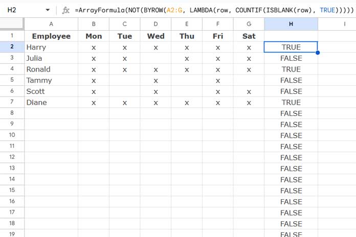

Formula Breakdown

We have created a custom unnamed LAMBDA function to use within the helper function BYROW, allowing us to apply this custom function to each row in a range.

Here is the custom unnamed function:

LAMBDA(row, COUNTIF(ISBLANK(row), TRUE))

The ISBLANK function returns TRUE for any blank cell in the current row, and the COUNTIF function counts the number of TRUE values. If any cell is empty, the count result will be greater than 0.

The BYROW function applies this LAMBDA function to each row in the range A2:G.

When you wrap this formula with NOT, rows where BYROW returns 0 (indicating no blank cells) will become TRUE, and other rows will become FALSE.

This helps us exclude rows with any blank cells during data manipulation.

Example 1: Exclude Rows with Any Blank Cells Using FILTER

When using the FILTER function, you can omit the ARRAYFORMULA wrapper from the formula above.

The example shows employee attendance for a week. I want to extract the employees who were fully present throughout the week.

=FILTER(
   A2:G, 
   NOT(BYROW(A2:G, LAMBDA(row, COUNTIF(ISBLANK(row), TRUE))))
)

This formula excludes rows with any blank cells while filtering the rows to a new range.

If you want to extract the employees who were absent on any day, simply remove the NOT function from the formula:

=FILTER(
   A2:G, 
   BYROW(A2:G, LAMBDA(row, COUNTIF(ISBLANK(row), TRUE)))
)

Example 2: Exclude Rows with Any Blank Cells Using COUNTIFS

Let’s consider the same sample data. How do you find how many employees were present for the whole week without taking any leave?

We can use the COUNTIFS function for this:

=COUNTIFS(
   ArrayFormula(NOT(BYROW(A2:G, LAMBDA(row, COUNTIF(ISBLANK(row), TRUE))))), TRUE
)

This COUNTIFS formula excludes rows with any blank cells while counting the rows where all columns have values.

If you want to count the employees who took leave on any day, you can use the following formula:

=COUNTIFS(
   ArrayFormula(NOT(BYROW(A2:G, LAMBDA(row, COUNTIF(ISBLANK(row), TRUE))))), FALSE, 
   A2:A, "<>"
)

This formula counts the FALSE values returned by the helper formula and ensures that A2:A is not blank. The second condition is necessary; otherwise, it will count blank rows, resulting in an incorrect total.

Resources

• Filter Out If the Entire Row Is Blank in Google Sheets
• Filter Out Blank Columns in Google Sheets Using Query Formula
• Lookup Header and Filter Non-Blanks in that Column in Google Sheets
• Count Blank Cells Row by Row in Google Sheets (COUNTBLANK Each Row)
• Sort Data but Keep Blank Rows in Excel and Google Sheets