We can use the Offset function to get dynamic ranges in SUMIF in Google Sheets. In this tutorial, we can learn that trick.

By the term “dynamic ranges,” I mean the range in a formula that accommodates values in any rows inserted later, just above or below the formula range.

So, this time, in this advanced SUMIF tutorial, you can learn how to use dynamic ranges in the SUMIF formula in Google Sheets.

How to Apply Dynamic Ranges in SUMIF Formula in Google Sheets

Let’s follow the below approach/steps to learn this.

1. Sample Data.
2. Basic SUMIF formula.
3. Creating a dynamic range for the SUMIF formula above.
4. Formula Explanation.

1. Sample Data

Here is my sample data for learning the dynamic ranges in a formula.

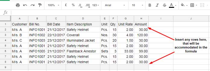
Here is the basic SUMIF formula.

2. Basic SUMIF Formula

=sumif(D2:D8,"Safety Helmet",H2:H8)

In this formula, D2:D8 is the range, “Safety Helmet” is the criterion, and H2:H8 is the Sum Range.

Syntax: SUMIF(range, criterion, [sum_range])

Result: 120.00

Now see what happens when you insert new rows above and bottom of our selected ranges in SUMIF.

The formula changes the ranges from D2:D8 to D3:D9 and H2:H8 to H3:H9. It excludes the newly added rows.

You can try using the Dollar Symbol to freeze the rows, as well as columns. But that doesn’t affect inserted rows.

3. How to Create a Dynamic Range for the Sumif Formula Above?

We can use Offset based dynamic ranges in SUMIF to overcome the above problem in Google Sheets.

In the above SUMIF formula, instead of the range D2:D8, we can use the below OFFSET formula.

offset(D1,1,0):offset(D9,-1,0)

For H2:H8, the alternative offset range is;

offset(H1,1,0):offset(H9,-1,0)

Now you can see how I’m going to apply dynamic ranges in the SUMIF formula in Google Sheets. Here is that formula.

=sumif(offset(D1,1,0):offset(D9,-1,0),"Safety Helmet",offset(H1,1,0):offset(H9,-1,0))

If you use this formula in the above example, there is no need for you to change the formula range manually.

When you insert new rows just above or below the formula range, they will be automatically included in the calculation.

4. Sumif Dynamic Range Formula Explanation

Before going to the formula explanation part, see what happens when I insert new rows above and below our data range.

Here our dynamic SUMIF formula using the Offset function returns the correct result in cell H14, whereas the usual SUMIF formula in cell H13 skips the inserted rows in the calculation.

There is nothing special in this dynamic formula. You are just replacing the range with the Offset.

See the Offset syntax.

OFFSET(cell_reference, offset_rows, offset_columns

Once again, see our basic/usual SUMIF formula and ranges.

=sumif(D2:D8,"Safety Helmet",H2:H8)

In SUMIF using Offset as ranges, D2:D8 is replaced by the below offset formula.

offset(D1,1,0):offset(D9,-1,0)

Instead of D2, here within Offset, I’ve used D1 as the cell reference and offset 1.

So here also, the cell reference is D2.

But the advantage is you can insert any number of rows just above D2. The Offset would include this in the dynamic ranges in SUMIF.

Similarly, in SUMIF, another cell reference is D8. But in dynamic SUMIF using Offset, it’s D9 and Offset -1.

So again, here also, the actual cell reference is pointing to D8.

The above points apply to the range H2:H8 also.

Resources

• REGEXMATCH in SUMIFS and Multiple Criteria Columns in Google Sheets.
• Multiple Sum Columns in SUMIF in Google Sheets.
• How to Sumif/Sumifs Excluding Duplicates in Google Sheets.
• Sumif Importrange in Google Sheets – Examples.
• Sum of Matrix Rows or Columns Using Sumif in Google Sheets.
• How to Use Sumif in Merged Cells in Google Sheets.