In a sorted range in Google Sheets, you can use my array formula to sum column B based on changes in the values in column A. Columns A and B are just examples; you can use any two columns.

The ultimate goal of the formula is to leave the total for each group in the last row of that group.

You need to enter the formula in an empty column in the first row of the first group. It will return totals in that column at the last row of each group.

I have two array formulas to sum column B based on value changes in column A. One uses the MAP Lambda function, while the other uses SUMIF and lookup functions. I prefer the latter because it performs better with large datasets.

However, we’ll start with a drag-down formula that places totals when the value in column A changes. Some of you may be looking for such a solution as well.

Non-Array (Drag-Down) Formula Approach

For consistency across all our examples, we will use the sample data in A1:B, where A1:B1 contains the field labels “Item” and “Qty.”

Column A determines the group change, and the first data row starts in A2. In C2, you can enter the following formula and drag it down as far as needed:

=IF($A2<>$A3, SUM($B$1:$B2)-SUM($C$1:$C1),"")

This formula sums column B based on changes in column A, placing the group total in the last row of each group.

When using this formula, replace:

• $A2 with the reference for the first row of the group column.
• $A3 with the reference for the second row of the group column.
• $B$1:$B2 with the range reference for the column you want to total, from the header to the first data row.
• $C$1:$C1 with the header row reference of the column as a range reference where you intend to apply the formula.

As mentioned earlier, there are two array formula approaches to place the total in a column when the value changes in another column. Based on the sample data above, you only need to enter one of them in cell C2. It will expand down and return the subtotal for each group in that column. Here they are.

Non-LAMBDA Array Formula to Sum Column B Based on Changes in Column A

To sum column B when the value changes in column A, insert the following formula in cell C2:

=ArrayFormula(IFNA(
   VLOOKUP(
      ROW(A2:A), 
      HSTACK(
         LOOKUP(UNIQUE(A2:A), A2:A, ROW(A2:A)), 
         UNIQUE(A2:A), SUMIF(A2:A, UNIQUE(A2:A), B2:B)
      ), 
      3, 0
   )
))

Where:

• A2:A is the range for the group column.
• B2:B is the range for the sum column.

When using this formula for different columns, you should modify these range references accordingly. No other changes are required.

Formula Breakdown

The formula has four key parts: UNIQUE, SUMIF, LOOKUP, and VLOOKUP.

Here are their roles in placing the group totals in the last row of each group:

Creating a Range for VLOOKUP:

• UNIQUE(A2:A) – Returns the unique categories in column A.
• LOOKUP(UNIQUE(A2:A), A2:A, ROW(A2:A)) – The LOOKUP function looks up the unique categories in A2:A and returns the row numbers of the last occurrence of those categories. Essentially, it returns the row numbers where we want to place the subtotals.
• SUMIF(A2:A, UNIQUE(A2:A), B2:B) – SUMIF sums the values in B2:B that match the unique categories in A2:A.

We combine these arrays using HSTACK to create a range where the first column contains the row numbers of the last occurrence of each category, along with the corresponding categories and the sum of those categories. Here’s that part:

HSTACK(
         LOOKUP(UNIQUE(A2:A), A2:A, ROW(A2:A)), 
         UNIQUE(A2:A), SUMIF(A2:A, UNIQUE(A2:A), B2:B)
      )

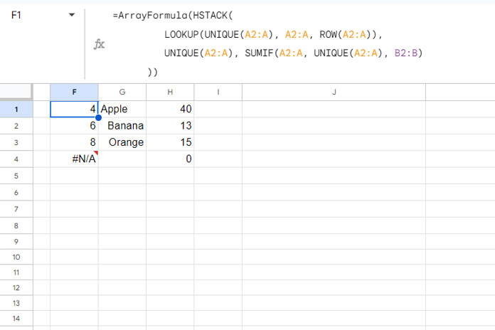
The VLOOKUP function looks up the row numbers from A2:A in the first column of this range and returns the corresponding values from the last column. This will place the totals in the last row of each group.

In this way, we can sum column B based on changes in values in column A and place the totals in column C in the last row.

LAMBDA Array Formula to Sum Column B Based on Changes in Column A

This is a completely different approach. Based on our sample data, you can use this formula in cell C2:

=IFNA(MAP(
   A2:A, 
   LAMBDA(val, 
      IF(ROW(val)=XMATCH(val, A2:A, 0, -1)+ROW(INDEX(A2:A, 1, 1))-1, 
         SUM(FILTER(B2:B, A2:A=val)),
      )
   )
))

This will return the sum of column B based on value changes in the group column A.

The logic of this formula is quite simple. Before we go into that, one thing to note is that if you have a very large volume of data, I wouldn’t recommend using this approach, as it may affect the performance of the sheet.

Formula Explanation

The MAP function maps each value in the array A2:A and returns a new value by applying a custom LAMBDA function. Within this LAMBDA function, each value is defined as val, and the function itself is structured as an IF logical test.

Here is the key part of the formula:

IF(ROW(val)=XMATCH(val, A2:A, 0, -1)+ROW(INDEX(A2:A, 1, 1))-1, 
   SUM(FILTER(B2:B, A2:A=val)),
)

This is an IF logical test that works as follows:

If the row number of the current element in the array, i.e., ROW(val), is equal to XMATCH(val, A2:A, 0, -1)+ROW(INDEX(A2:A, 1, 1))-1:

• XMATCH(val, A2:A, 0, -1) finds the last occurrence of the category (val) in column A and returns its relative position.
• +ROW(INDEX(A2:A, 1, 1))-1 part converts the relative position to the actual row number, allowing the formula to identify the last row number of the category.

Then it returns:

SUM(FILTER(B2:B, A2:A=val)): The FILTER function filters column B to match the current element in column A and sums the total.

Do you want a custom function to aggregate (sum, average, etc.) a column based on changes in values in another column? If so, please refer to the resource section below.

Resources

• AT_EACH_CHANGE Named Functions in Google Sheets
• Highlight Rows When the Value Changes in Any Column
• How to Find the Last Row in Each Group in Google Sheets
• 4 Formulas to Last Row Lookup and Array Result in Google Sheets
• Get the First and Last Row Numbers of Items in Google Sheets
• Get the First or Last Row/Column in a New Google Sheets Table