This tutorial guides you through MAXIFS array formulas in Google Sheets, providing step-by-step instructions, real-world examples, and valuable tips.
It’s important to note that the MAXIFS function may not automatically expand or spill results when used with the ARRAYFORMULA function. In such cases, consider utilizing the MAP lambda function for expansion.
Alternatively, you can explore alternative approaches like the SORT+SORTN combination or QUERY, depending on your specific requirements.
Whether you’re a beginner or an experienced user, this tutorial ensures you acquire the knowledge to leverage MAXIFS effectively for enhanced data analysis.
We will utilize the following sample data to evaluate MAXIFS array formulas in Google Sheets:
| Name | Attempt | Length (Score) in Mtr. |
| Maria | 1st | 5.72 |
| Maria | 2nd | 5.58 |
| Maria | 3rd | 5.81 |
| John | 1st | 5.25 |
| John | 2nd | 5.4 |
| John | 3rd | 5.31 |
| Aisha | 1st | 5.6 |
| Aisha | 2nd | 5.65 |
| Aisha | 3rd | 5.56 |
The provided sample data illustrates the scores (lengths achieved) of three participants across three attempts in a long jump event. Feel free to copy and paste it into cell range A1:C10 in your Google Sheets file. Once done, we can move on to the formulas.
MAXIFS and MAP Lambda for Array Results (Testing Multiple Criteria in Single Column)
The goal is to find the highest score for each participant in a single MAXIFS formula, regardless of their attempts.
Participant names are located in the range A2:A, and their corresponding scores are in the range C2:C, with the first row (A1:C1) serving as field labels (row headers).
Steps:
- Enter this formula in cell E2:
=UNIQUE(A2:A)This generates a list of unique participant names in E2:E4 (or further down if more participants exist). - Array Formula for Maximum Scores (F2):
=MAP(E2:E4, LAMBDA(r, MAXIFS(C2:C, A2:A, r)))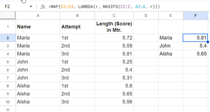
Formula Break Down:
- We employ the MAP Lambda function to apply a MAXIFS function to a specific range that contains multiple criteria (unique participant names).
MAXIFS(C2:C, A2:A, r)– This is the MAXIFS formula whererrepresents the current element in the array E2:E4, specified in the MAP.- C2:C represents the
range, A2:A is thecriteria_range1, andris thecriterion1.
- C2:C represents the
- So,
rwill be E2 in the first row, E3 in the second row, and E4 in the third row. - The MAP iterates over the array E2:E4, allowing us to convert a MAXIFS formula into an array formula in Google Sheets.
MAXIFS and MAP Lambda for Array Results (Testing Multiple Criteria in Multiple Columns)
Once you’ve mastered the MAXIFS array formula with a single criterion column, adapting it to handle multiple criteria columns becomes straightforward.
Here, the objective is to identify the highest score of each participant in their final (3rd) attempt. Follow these steps:
- Enter
=UNIQUE(A2:A)(the same earlier UNIQUE formula) in cell E2. - Enter the text “3rd” in cells F2, F3, and F4.
- In cell G2, insert the following MAXIFS array formula that utilizes the MAP Lambda function:
=MAP(E2:E4, F2:F4, LAMBDA(x, y, MAXIFS(C2:C, A2:A, x, B2:B, y)))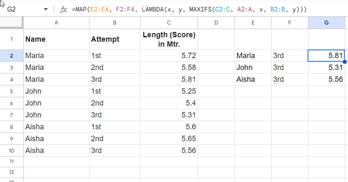
This formula iterates through each name-attempt pair, finding the maximum score using MAXIFS within the lambda function.
In MAXIFS, C2:C represents the range, A2:A is the criteria_range1, x is the criterion1, B2:B is the criteria_range2, and y is the criterion2.
Here, in the first row, x represents E2, and y represents F2. In the second row, x corresponds to E3, and y to F3. In the third row, x is linked to E4, and y to F4. The MAP function aids in iterating through each criteria range.
Exploring QUERY Function as an Alternative to MAXIFS Array Formulas
When seeking the highest scores based on multiple criteria in one go, don’t limit yourself to MAXIFS—consider the powerful option of using QUERY.
In QUERY, the MAX aggregation function allows you to retrieve the maximum value from a specific column while applying criteria in one or more columns and grouping the results. The output retains a structured table format.
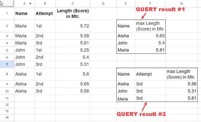
For instance, to obtain the maximum scores of each participant regardless of their attempts, utilize the following QUERY formula:
=QUERY(A1:C, "select A, max(C) where A is not null group by A", 1)Explanation:
A1:C: The data to be queried (including the header row).select A, max(C): Indicates that the output includes values from column A and the maximum value from column C.where A is not null: Specifies the criterion that the data should include values in column A that are not equal to blank.group by A: Groups the results by unique values in column A.
To retrieve the maximum scores of each participant on their 3rd attempt, use the following QUERY formula:
=QUERY(A1:C, "select A, B, max(C) where B='3rd' group by A, B", 1)Explanation:
A1:C: The data to be queried (including the header row).select A, B, max(C): Indicates that the output includes values from columns A, and B, and the maximum value from column C.where B='3rd': Specifies the criterion that the data should meet where values in column B are equal to ‘3rd’.group by A, B: Groups the results by unique values in columns A and B.
In short, the QUERY function is one of the perfect alternatives to MAXIFS array formulas.
Exploring SORTN Function as an Alternative to MAXIFS Array Formulas
The SORT+SORTN combo is another option to replace a MAXIFS array formula.
The logic is quite simple here. We will use the SORT function to arrange the table by the score in descending order. Then, we will use SORTN to return the first n rows after removing duplicate rows with respect to the name.
Sometimes you may additionally need to apply the FILTER function before these operations.
Let’s explore two examples so that you can understand how you can replace MAXIFS array formulas using this combo in Google Sheets.
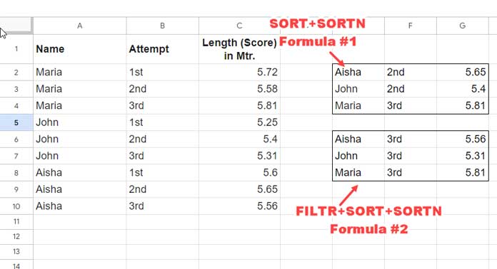
Formula to Return the Maximum Score of Each Participant:
=SORTN(SORT(A2:C, 3, 0), 9^9, 2, 1, TRUE)The SORT function sorts the third column (score) in descending order.
The SORTN returns 9^9 (an arbitrarily large number) rows, removing duplicates (tie mode #2). It sorts the result by column 1 in ascending order.
Formula to Return the Maximum Score of Each Participant In their 3rd Attempt:
=SORTN(SORT(FILTER(A2:C, B2:B="3rd"), 3, 0), 9^9, 2, 1, TRUE)The FILTER function filters the table matching “3rd” in B2:B. The rest of the SORT and SORTN operations are similar to the first formula.
These formulas provide excellent alternatives to MAXIFS array formulas.


