Tracking the highest value per week in Google Sheets is essential for analyzing trends—whether you’re monitoring sales, stock prices, or website traffic. But how do you quickly extract the weekly max without manually sorting through your data?
In this guide, I’ll show you simple yet powerful formulas to get the max per week in Google Sheets using the key functions MAXIFS, QUERY, and SORTN. Out of the three, I recommend SORTN for its efficiency.
By the end, you’ll be able to:
- Find the maximum value for each week automatically
- Group and analyze weekly data efficiently
- Choose the best method based on your dataset
Let’s dive in!
Why Pivot Tables Aren’t Ideal for Finding Max Per Week in Google Sheets
As a side note, you can’t use a Pivot Table directly to find the max per week in Google Sheets. To make it work, you’d need one or two helper columns—either separating the week number and year or combining them into a single column.
Since this adds extra steps, it’s much easier to stick with my formula-based approaches, which allow you to extract the maximum value per week in Google Sheets without additional setup.
Sample Data
We have the following sales data in A1:B:
| Date | Sales |
| 01/01/2025 | 9 |
| 02/01/2025 | 10 |
| 03/01/2025 | 15 |
| 04/01/2025 | 10 |
| 06/01/2025 | 4 |
| 07/01/2025 | 3 |
| 08/01/2025 | 19 |
| 09/01/2025 | 1 |
| 10/01/2025 | 12 |
| 11/01/2025 | 10 |
Let’s find the max sales per week.
Max Per Week Using the SORTN Function in Google Sheets
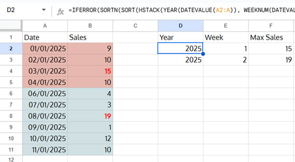
You can use the following formula in D2 to get the max sales per week:
=IFERROR(SORTN(SORT(HSTACK(YEAR(DATEVALUE(A2:A)), WEEKNUM(DATEVALUE(A2:A), 2), B2:B), 1, 1, 2, 1, 3, 0), 9^9, 2, 1, TRUE, 2, TRUE))Formula Adjustments
- The formula considers a Monday–Sunday week. If you want a Sunday–Saturday week, replace
2inWEEKNUMwith1. - If you want a different starting day, refer to my WEEKNUM function guide.
- Replace
A2:Awith your date range andB2:Bwith the sales column.
Formula Output
Formula Explanation
HSTACK(YEAR(DATEVALUE(A2:A)), WEEKNUM(DATEVALUE(A2:A), 2), B2:B): Creates a three-column array with year, week number, and sales.SORT(..., 1, 1, 2, 1, 3, 0): Sorts by year and week in ascending order and sales in descending order.SORTN(..., 9^9, 2, 1, TRUE, 2, TRUE): Removes duplicates, keeping only the maximum sales per week.
Find the Maximum Value Per Week Using QUERY
You can use the same three-column array from SORTN with QUERY. Here’s the formula:
=QUERY(ARRAYFORMULA(HSTACK(YEAR(DATEVALUE(A2:A)), WEEKNUM(DATEVALUE(A2:A), 2), B2:B)), "SELECT Col1, Col2, MAX(Col3) WHERE Col1 IS NOT NULL GROUP BY Col1, Col2 LABEL MAX(Col3)''")How Does This Formula Work?
ARRAYFORMULA(HSTACK(YEAR(DATEVALUE(A2:A)), WEEKNUM(DATEVALUE(A2:A), 2), B2:B)): Converts the dataset into a structured array.QUERY(...): Groups by year and week and returns the maximum sales per week.
Max Per Week Using MAXIFS in Google Sheets
This approach does not generate a weekly summary but instead places the max value within each row’s corresponding week.
Formula for C2 (Drag Down):
=ArrayFormula(MAXIFS($B$2:$B, YEAR($A$2:$A), YEAR(A2), WEEKNUM($A$2:$A, 2), WEEKNUM(A2, 2)))- The
MAXIFSfunction returns the max sales value within each row’s week. - It matches year and week number across the dataset.
Auto-Expanding Formula Using MAP:
=ArrayFormula(MAP(A2:A, LAMBDA(dt, IF(dt="",,MAXIFS(B2:B, YEAR(A2:A), YEAR(dt), WEEKNUM(A2:A, 2), WEEKNUM(dt, 2))))))This version automatically expands as new data is added.
Summary
You now have three methods to find the max per week in Google Sheets:
- SORTN – Best for structured summaries.
- QUERY – Great for grouping data.
- MAXIFS – Works within each row.


