We can follow three approaches to calculate the quarterly average in Google Sheets: QUERY, Pivot Table, and AVERAGEIFS.

Both QUERY and Pivot Table methods do not necessitate a helper column, whereas AVERAGEIFS requires a helper column containing dates converted to quarters.

If your data spans more than one year, you can modify all the formulas and the Pivot Table to calculate the average, grouped by year and quarter. I’ll include these tips in this guide as well.

Calculating Average by Quarter Using the QUERY Function

Enter the sample data below into cells A1:B, where column A contains sales dates, and column B contains sales amounts.

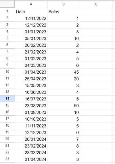
As evident from the data, it spans three years. To calculate the average, grouped by quarter, using the QUERY function, you must specify the desired year (e.g., 2023) within the query string, as illustrated below:

=QUERY(A1:B, "SELECT QUARTER(A), AVG(B) WHERE YEAR(A) = 2023 GROUP BY QUARTER(A)", 1)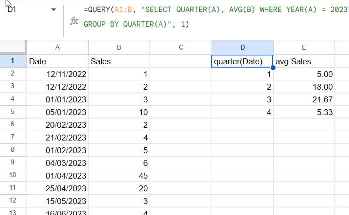

This formula adheres to the QUERY syntax:

QUERY(data, query, [headers])

Where:

• data: A1:B
• query: "SELECT QUARTER(A), AVG(B) WHERE YEAR(A) = 2023 GROUP BY QUARTER(A)"
  • SELECT QUARTER(A), AVG(B): Selects the quarter of the date in column A and calculates the average of corresponding values in column B.
  • WHERE YEAR(A) = 2023: Filters the data to include only rows where the year in column A is 2023.
  • GROUP BY QUARTER(A): The grouping is necessary for obtaining quarterly averages. If you just use "SELECT AVG(B)", it returns the average of values in column B overall. However, since you selected QUARTER(A), grouping by quarter is essential to get the average for each quarter separately.
• headers: 1

Adjustments in the QUERY Formula for Calculating Average by Year-Quarter:

To calculate the average, grouped by year and quarter, using the provided QUERY formula, make the following three changes:

1. Replace the filter condition WHERE YEAR(A) = 2023 with WHERE A IS NOT NULL.
2. Replace SELECT QUARTER(A) with SELECT YEAR(A), QUARTER(A).
3. Replace GROUP BY QUARTER(A) with GROUP BY YEAR(A), QUARTER(A).

Adjusted Formula:

=QUERY(A1:B, "SELECT YEAR(A), QUARTER(A), AVG(B) WHERE A IS NOT NULL GROUP BY YEAR(A), QUARTER(A)", 1)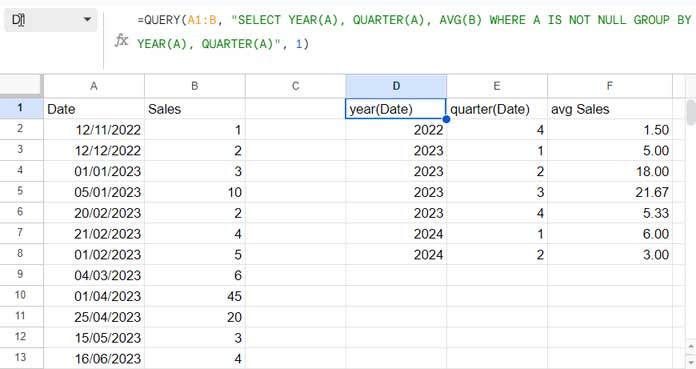

Calculating Average by Quarter Using the Pivot Table

In the early stages of Google Sheets, pivot date grouping was not available within Pivot Tables. Later, developers included this feature.

Let’s explore how to use the Pivot Table in Google Sheets to calculate the average grouped by quarter.

1. Click on “Insert” > “Pivot Table.”
2. Enter “A:B” in the field below “Data range.”
3. Select “Existing Sheet” and enter “D1” in the field below.
4. Click “Create.”
5. In the Pivot Table editor panel, drag and drop the ‘Date’ field below Rows.
6. Drag and drop the ‘Sales’ field below Values and select “AVERAGE” under “Summarize by.”
7. Drag and drop the ‘Date’ field below Filters. Under “Status,” click the drop-down, select “Filter by conditions,” then choose “Custom formula is,” and enter the following formula: =YEAR(Date)=2023.
8. Click “OK.”
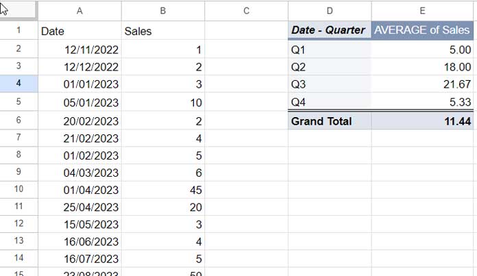
9. Right-click on any date in column D in the Pivot Table report. From the context menu, select “Create pivot date group” and then choose “Quarter.”

Adjustments in the Pivot Table Editor Panel for Calculating Average by Year-Quarter

To calculate the average grouped by year and quarter in the above Pivot Table, follow these two adjustments:

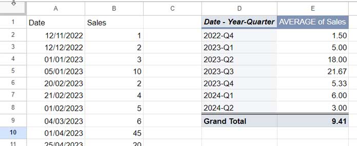
Right-click on Q1, Q2, Q3, or Q4 in column D, then select “Create pivot date group” and choose “Year-Quarter.”

Click on the pencil icon at the bottom left corner of the Pivot Table to open the sidebar editor panel. Scroll down to the bottom, and within the FILTERS section, replace the earlier custom formula with the following one: =DATEVALUE(Date)>0.

Calculating Average by Quarter Using the AVERAGEIFS Function

A helper column is needed for this method, unlike the previous two approaches. In cell C2, use the following formula to assign quarters to the dates:

=ArrayFormula(IFERROR("Q"&INT((MONTH(DATEVALUE(A2:A))+2)/3)))

This array formula will return the quarters for all dates in the rows.

In the above formula, the INT((MONTH(DATEVALUE(A2:A))+2)/3) part converts the month to a quarter number (1, 2, 3, or 4). The DATEVALUE is used in the formula to handle blank cells, ensuring it returns an error for them. Otherwise, if a cell is blank, the MONTH function would return 12 as the month number, and subsequently, the formula would return 4 as the quarter.

We have prepended “Q” to the numbers obtained above using the ampersand. The IFERROR function is used to handle any errors that might be returned by the formula, ensuring a clean output.

Note: Date functions require array formula support when used in a range.

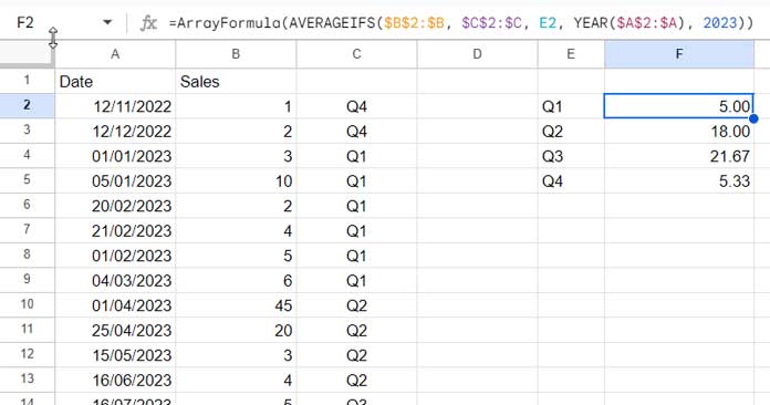
In cell E2, enter the below formula to get unique quarters sorted in ascending order:

=SORT(UNIQUE(C2:C))

In cell F2, use the following AVERAGEIFS formula:

=ArrayFormula(AVERAGEIFS($B$2:$B, $C$2:$C, E2, YEAR($A$2:$A), 2023))

It follows the below syntax:

AVERAGEIFS(average_range, criteria_range1, criterion1, [criteria_range2, …], [criterion2, …])

Where:

• average_range: $B$2:$B
• criteria_range1: $C$2:$C
• criterion1: E2
• criteria_range2: YEAR($A$2:$A)
• criterion2: 2023

Click and drag the blue square (fill handle) in the lower-right corner of cell F2 to fill the remaining cells with quarterly averages.

These steps guide you through calculating the average grouped by quarter using the AVERAGEIFS function with a helper column.

Adjustments in the Formulas for Calculating Average by Year-Quarter

To make the necessary adjustments for calculating the average grouped by year and quarter, follow these two changes:

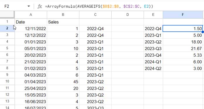
Replace the formula in cell C2, the helper column, with the following one, which prepends the year to the quarter label:

=ArrayFormula(IFERROR(YEAR(DATEVALUE(A2:A))&"-Q"&INT((MONTH(DATEVALUE(A2:A))+2)/3)))

This array formula will assign year-quarter labels to the dates.

Replace the formula in cell F2 with the following one:

=AVERAGEIFS($B$2:$B, $C$2:$C, E2)

Drag this formula down as far as you want.

Selecting the Best Option from the Three Choices

The Pivot Table stands out as the most flexible option among the three, allowing easy switching between quarter, year-quarter, month, year, and year-month summary reports.

I don’t recommend using AVERAGEIFS due to its multiple steps and the need for careful execution.

For beginners, the Pivot Table is the preferred choice. If you aim to learn functions, opt for AVERAGEIFS.

I prefer QUERY. Choose QUERY if you don’t need to customize the result header. However, if customization is essential, consider exploring the LABEL clause.

Resources

Interested in exploring more about quarterly-based calculations beyond calculating averages by quarter? Check out these guides:

1. Group Dates in Pivot Table in Google Sheets (Month, Quarter, and Year)
2. Formula to Group Dates by Quarter in Google Sheets
3. Query to Create Daily/Weekly/Monthly/Quarterly/Yearly Report Summary in Google Sheets
4. Extract Quarter from a Date in Google Sheets – Formula Options
5. Query Quarter Function in Non-Calendar Fiscal Year Data (Google Sheets)
6. Convert Dates To Fiscal Quarters in Google Sheets
7. Current Quarter and Previous Quarter Calculations in Google Sheets