If financial reporting in your organization follows a fiscal year instead of the calendar year, you may find it challenging to group data properly. This is because fiscal years may not align with standard calendar years. If you need to categorize dates into fiscal quarters (Q1, Q2, Q3, Q4) and fiscal years (FY23, FY24, etc.), Google Sheets can automate this process using formulas.

This tutorial will guide you through how to convert dates to fiscal quarters and years, whether your fiscal year starts in January, April, or any other month. You can use the following dynamic formula for this:

=LET(dt, A2, start, 1, fqtr, INT(MOD(MONTH(dt)-start, 12)/3+1), fyrs, YEAR(dt)-(MONTH(dt)<start), fyre, RIGHT(YEAR(dt)+(MONTH(dt)>=start), 2), "Q"&fqtr&" FY "&fyrs&IF(start=1,,"-"&fyre))

When using this formula, replace A2 (dt) with the cell containing the date you want to convert to a fiscal quarter and year, and replace 1 (start) with the fiscal year start month number.

Example: Convert Dates to Fiscal Quarters and Years in Google Sheets

Assume you have dates in column A and your financial year starts in April and ends in March, spanning two calendar years.

Enter the following formula in cell B2:

=LET(dt, A2, start, 4, fqtr, INT(MOD(MONTH(dt)-start, 12)/3+1), fyrs, YEAR(dt)-(MONTH(dt)<start), fyre, RIGHT(YEAR(dt)+(MONTH(dt)>=start), 2), "Q"&fqtr&" FY "&fyrs&IF(start=1,,"-"&fyre))

Then, navigate to B2, and if not already selected, hover your mouse over the fill handle at the bottom right corner. When it turns into a cross sign, click and drag it down as far as needed.

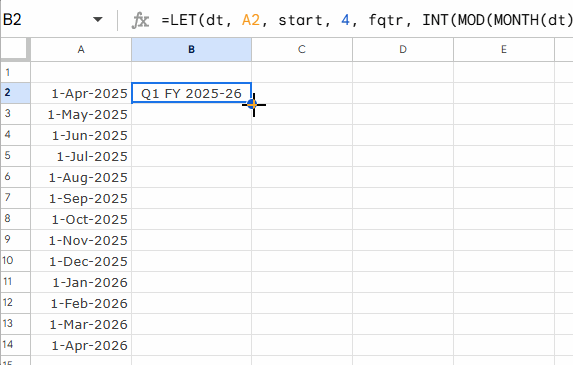
• If the date in A2 is 26/04/2025, the formula will return “Q1 FY 2025-26”.
• If the date in A2 is 18/03/2026, the formula will return “Q4 FY 2025-26”.
• If your financial year starts in January and ends in December (matching the calendar year), the formula will return “Q1 FY 2025” for 15/01/2025.

This means the above formula is fully flexible and can convert dates to financial quarters regardless of whether your fiscal year aligns with the calendar year, financial year, or a custom fiscal year.

Using the Fiscal Quarter Formula as an Array Formula

You can convert an entire column of dates to fiscal quarters using an array formula. However, when doing so, you need to handle empty cells appropriately.

Empty cells usually contain 0, which may be interpreted as a date serial and converted to 30/12/1899. As a result, the fiscal quarter formula may assign incorrect values. You can avoid this issue using the following modified formula:

=ArrayFormula(LET(dt, A2:A, start, 1, fqtr, INT(MOD(MONTH(dt)-start, 12)/3+1), fyrs, YEAR(dt)-(MONTH(dt)<start), fyre, RIGHT(YEAR(dt)+(MONTH(dt)>=start), 2), IF(dt="",,"Q"&fqtr&" FY "&fyrs&IF(start=1,,"-"&fyre)))))

Replace A2:A with the date range and 1 (start) with the fiscal quarter start month number.

Formula Explanation

The formula dynamically converts dates to fiscal quarters and years using three key components:

1. Finding the Fiscal Quarter from a Date (fqtr)

INT(MOD(MONTH(dt)-start, 12)/3+1)

• MONTH(dt): Extracts the month number from the date in A2.
• MONTH(A2)-start: Adjusts the month number based on the fiscal start month.
• MOD(MONTH(dt)-start, 12): Keeps the values within a 12-month cycle (0-11).
• MOD(…, 12)/3: Groups the adjusted month numbers into quarters.
• INT(…)+1: Ensures whole numbers and starts quarters from Q1 instead of Q0.

2. Finding the Fiscal Starting Year (fyrs)

YEAR(dt)-(MONTH(dt)<start)

• (MONTH(dt)<start): Returns 1 (TRUE) if the month is before the fiscal start; otherwise, 0 (FALSE).
• Subtracting this value from YEAR(dt) gives the correct fiscal start year.

For example, if the fiscal year starts in April:

• 1 April 2024 ➤ Fiscal Year Start: 2024
• 1 March 2025 ➤ Fiscal Year Start: 2024

3. Finding the Fiscal Ending Year (fyre)

RIGHT(YEAR(dt)+(MONTH(dt)>=start), 2)

• (MONTH(dt)>=start): Returns 1 if the month is greater than or equal to the fiscal start; otherwise, 0.
• Adding this to YEAR(dt) provides the fiscal ending year.

For example:

• 1 April 2024 ➤ Fiscal Year End: 2025
• 1 March 2025 ➤ Fiscal Year End: 2025

Conclusion

This formula effectively converts dates to fiscal quarters and years in Google Sheets, allowing flexibility for different fiscal year start months. It is useful for financial reporting and analysis.

Related Resources

• Group Dates in Pivot Table in Google Sheets (Month, Quarter, and Year)
• How to Group Dates by Quarter in Google Sheets
• Query Daily, Weekly, Monthly, Quarterly, and Yearly Reports in Google Sheets
• Extract Quarter from a Date in Google Sheets: Formulas
• Query Quarter Function in Non-Calendar Fiscal Year Data (Google Sheets)
• Current Quarter and Previous Quarter Calculation in Google Sheets
• How to Calculate Average by Quarter in Google Sheets
• Sum By Quarter in Excel: New and Efficient Techniques